Multipoint Optimization
To simulate multiple flight conditions in a single analysis or optimization, you can add multiple AeroPoint or AerostructPoint groups to the problem. This allows you to analyze the performance of the aircraft at multiple flight conditions simultaneously, such as at different cruise and maneuver conditions.
Aerodynamic Optimization Example
We optimize the aircraft at two cruise flight conditions below.
import numpy as np
import openmdao.api as om

from openaerostruct.meshing.mesh_generator import generate_mesh
from openaerostruct.geometry.geometry_group import Geometry
from openaerostruct.aerodynamics.aero_groups import AeroPoint
from openaerostruct.integration.multipoint_comps import MultiCD

# Create a dictionary to store options about the surface
mesh_dict = {
    "num_y": 5,
    "num_x": 3,
    "wing_type": "CRM",
    "symmetry": True,
    "num_twist_cp": 5,
    "span_cos_spacing": 0.0,
}

mesh, twist_cp = generate_mesh(mesh_dict)

surf_dict = {
    # Wing definition
    "name": "wing",  # name of the surface
    "symmetry": True,  # if true, model one half of wing
    # reflected across the plane y = 0
    "S_ref_type": "wetted",  # how we compute the wing area,
    # can be 'wetted' or 'projected'
    "fem_model_type": "tube",
    "mesh": mesh,
    "twist_cp": twist_cp,
    # Aerodynamic performance of the lifting surface at
    # an angle of attack of 0 (alpha=0).
    # These CL0 and CD0 values are added to the CL and CD
    # obtained from aerodynamic analysis of the surface to get
    # the total CL and CD.
    # These CL0 and CD0 values do not vary wrt alpha.
    "CL0": 0.0,  # CL of the surface at alpha=0
    "CD0": 0.015,  # CD of the surface at alpha=0
    # Airfoil properties for viscous drag calculation
    "k_lam": 0.05,  # percentage of chord with laminar
    # flow, used for viscous drag
    "t_over_c_cp": np.array([0.15]),  # thickness over chord ratio (NACA0015)
    "c_max_t": 0.303,  # chordwise location of maximum (NACA0015)
    # thickness
    "with_viscous": True,  # if true, compute viscous drag
    "with_wave": False,  # if true, compute wave drag
}

surfaces = [surf_dict]

n_points = 2

# Create the problem and the model group
prob = om.Problem()

indep_var_comp = om.IndepVarComp()
indep_var_comp.add_output("v", val=248.136, units="m/s")
indep_var_comp.add_output("alpha", val=np.ones(n_points) * 6.64, units="deg")
indep_var_comp.add_output("Mach_number", val=0.84)
indep_var_comp.add_output("re", val=1.0e6, units="1/m")
indep_var_comp.add_output("rho", val=0.38, units="kg/m**3")
indep_var_comp.add_output("cg", val=np.zeros((3)), units="m")

prob.model.add_subsystem("prob_vars", indep_var_comp, promotes=["*"])

# Loop over each surface and create the geometry groups
for surface in surfaces:
    # Get the surface name and create a group to contain components only for this surface.
    name = surface["name"]
    geom_group = Geometry(surface=surface)

    # Add geom_group to the problem with the name of the surface.
    prob.model.add_subsystem(name + "_geom", geom_group)

# Loop through and add a certain number of aero points
for i in range(n_points):
    # Create the aero point group and add it to the model
    aero_group = AeroPoint(surfaces=surfaces)
    point_name = "aero_point_{}".format(i)
    prob.model.add_subsystem(point_name, aero_group)

    # Connect flow properties to the analysis point
    prob.model.connect("v", point_name + ".v")
    prob.model.connect("alpha", point_name + ".alpha", src_indices=[i])
    prob.model.connect("Mach_number", point_name + ".Mach_number")
    prob.model.connect("re", point_name + ".re")
    prob.model.connect("rho", point_name + ".rho")
    prob.model.connect("cg", point_name + ".cg")

    # Connect the parameters within the model for each aero point
    for surface in surfaces:
        name = surface["name"]

        # Connect the drag coeff at each point to the multi_CD component, which does the summation.
        prob.model.connect(point_name + ".CD", "multi_CD." + str(i) + "_CD")

        # Connect the mesh from the geometry component to the analysis point
        prob.model.connect(name + "_geom.mesh", point_name + "." + name + ".def_mesh")

        # Perform the connections with the modified names within the 'aero_states' group.
        prob.model.connect(name + "_geom.mesh", point_name + ".aero_states." + name + "_def_mesh")
        prob.model.connect(name + "_geom.t_over_c", point_name + "." + name + "_perf." + "t_over_c")

prob.model.add_subsystem("multi_CD", MultiCD(n_points=n_points), promotes_outputs=["CD"])

prob.driver = om.ScipyOptimizeDriver()
prob.driver.options["tol"] = 1e-9

# Setup problem and add design variables, constraint, and objective
# design variables are the wing twist and angle-of-attack at each point.
prob.model.add_design_var("alpha", lower=-15, upper=15)
prob.model.add_design_var("wing_geom.twist_cp", lower=-5, upper=8)

# set different target CL value at each point.
prob.model.add_constraint("aero_point_0.wing_perf.CL", equals=0.45)
prob.model.add_constraint("aero_point_1.wing_perf.CL", equals=0.5)

# objective is the sum of CDs at each point.
prob.model.add_objective("CD", scaler=1e4)

# Set up the problem and run optimization.
prob.setup()
prob.run_driver()
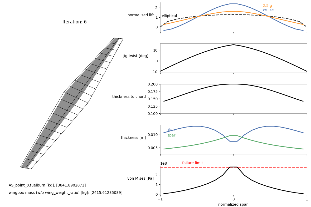
Aerostructural Optimization Example (Q400)
This is an additional example of a multipoint aerostructural optimization with the wingbox model using a wing based on the Bombardier Q400. Here we also create a custom mesh instead of using one provided by OpenAeroStruct. Make sure you go through the Aerostructural Optimization with Wingbox before trying to understand this example.
"""
This example script can be used to run a multipoint aerostructural optimization
for a wing based on the Bombardier Q400 with the wingbox model.
We create a custom mesh for this wing in this script.
The fuel burn from the cruise flight-point is the objective function and a 2.5g
maneuver flight-point is used for the structural sizing.
After running the optimization, use the 'plot_wingbox.py' script in the utils/
directory (e.g., as 'python ../utils/plot_wingbox.py aerostruct.db' if running
from this directory) to visualize the results.
This visualization script is based on the plot_wing.py script.
It's still under development and will probably not work as it is for other types of
cases for now.
"""

import numpy as np

from openaerostruct.integration.aerostruct_groups import AerostructGeometry, AerostructPoint
from openaerostruct.structures.wingbox_fuel_vol_delta import WingboxFuelVolDelta
import openmdao.api as om

# Provide coordinates for a portion of an airfoil for the wingbox cross-section as an nparray with dtype=complex (to work with the complex-step approximation for derivatives).
# These should be for an airfoil with the chord scaled to 1.
# We use the 10% to 60% portion of the NASA SC2-0612 airfoil for this case
# We use the coordinates available from airfoiltools.com. Using such a large number of coordinates is not necessary.
# The first and last x-coordinates of the upper and lower surfaces must be the same

# fmt: off
upper_x = np.array([0.1, 0.11, 0.12, 0.13, 0.14, 0.15, 0.16, 0.17, 0.18, 0.19, 0.2, 0.21, 0.22, 0.23, 0.24, 0.25, 0.26, 0.27, 0.28, 0.29, 0.3, 0.31, 0.32, 0.33, 0.34, 0.35, 0.36, 0.37, 0.38, 0.39, 0.4, 0.41, 0.42, 0.43, 0.44, 0.45, 0.46, 0.47, 0.48, 0.49, 0.5, 0.51, 0.52, 0.53, 0.54, 0.55, 0.56, 0.57, 0.58, 0.59, 0.6], dtype="complex128")
lower_x = np.array([0.1, 0.11, 0.12, 0.13, 0.14, 0.15, 0.16, 0.17, 0.18, 0.19, 0.2, 0.21, 0.22, 0.23, 0.24, 0.25, 0.26, 0.27, 0.28, 0.29, 0.3, 0.31, 0.32, 0.33, 0.34, 0.35, 0.36, 0.37, 0.38, 0.39, 0.4, 0.41, 0.42, 0.43, 0.44, 0.45, 0.46, 0.47, 0.48, 0.49, 0.5, 0.51, 0.52, 0.53, 0.54, 0.55, 0.56, 0.57, 0.58, 0.59, 0.6], dtype="complex128")
upper_y = np.array([ 0.0447,  0.046,  0.0472,  0.0484,  0.0495,  0.0505,  0.0514,  0.0523,  0.0531,  0.0538, 0.0545,  0.0551,  0.0557, 0.0563,  0.0568, 0.0573,  0.0577,  0.0581,  0.0585,  0.0588,  0.0591,  0.0593,  0.0595,  0.0597,  0.0599,  0.06,    0.0601,  0.0602,  0.0602,  0.0602,  0.0602,  0.0602,  0.0601,  0.06,    0.0599,  0.0598,  0.0596,  0.0594,  0.0592,  0.0589,  0.0586,  0.0583,  0.058,   0.0576,  0.0572,  0.0568,  0.0563,  0.0558,  0.0553,  0.0547,  0.0541], dtype="complex128")  # noqa: E201, E241
lower_y = np.array([-0.0447, -0.046, -0.0473, -0.0485, -0.0496, -0.0506, -0.0515, -0.0524, -0.0532, -0.054, -0.0547, -0.0554, -0.056, -0.0565, -0.057, -0.0575, -0.0579, -0.0583, -0.0586, -0.0589, -0.0592, -0.0594, -0.0595, -0.0596, -0.0597, -0.0598, -0.0598, -0.0598, -0.0598, -0.0597, -0.0596, -0.0594, -0.0592, -0.0589, -0.0586, -0.0582, -0.0578, -0.0573, -0.0567, -0.0561, -0.0554, -0.0546, -0.0538, -0.0529, -0.0519, -0.0509, -0.0497, -0.0485, -0.0472, -0.0458, -0.0444], dtype="complex128")
# fmt: on

# Here we create a custom mesh for the wing
# It is evenly spaced with nx chordwise nodal points and ny spanwise nodal points for the half-span

span = 28.42  # wing span in m
root_chord = 3.34  # root chord in m

nx = 3  # number of chordwise nodal points (should be odd)
ny = 11  # number of spanwise nodal points for the half-span

# Initialize the 3-D mesh object. Chordwise, spanwise, then the 3D coordinates.
mesh = np.zeros((nx, ny, 3))

# Start away from the symmetry plane and approach the plane as the array indices increase.
# The form of this 3-D array can be very confusing initially.
# For each node we are providing the x, y, and z coordinates.
# x is chordwise, y is spanwise, and z is up.
# For example (for a mesh with 5 chordwise nodes and 15 spanwise nodes for the half wing), the node for the leading edge at the tip would be specified as mesh[0, 0, :] = np.array([1.1356, -14.21, 0.])
# and the node at the trailing edge at the root would be mesh[4, 14, :] = np.array([3.34, 0., 0.]).
# We only provide the left half of the wing because we use symmetry.
# Print the following mesh and elements of the mesh to better understand the form.

mesh[:, :, 1] = np.linspace(-span / 2, 0, ny)
mesh[0, :, 0] = 0.34 * root_chord * np.linspace(1.0, 0.0, ny)
mesh[2, :, 0] = root_chord * (np.linspace(0.4, 1.0, ny) + 0.34 * np.linspace(1.0, 0.0, ny))
mesh[1, :, 0] = (mesh[2, :, 0] + mesh[0, :, 0]) / 2

# print(mesh)

surf_dict = {
    # Wing definition
    "name": "wing",  # name of the surface
    "symmetry": True,  # if true, model one half of wing
    "S_ref_type": "wetted",  # how we compute the wing area,
    # can be 'wetted' or 'projected'
    "mesh": mesh,
    "twist_cp": np.array([6.0, 7.0, 7.0, 7.0]),
    "fem_model_type": "wingbox",
    "data_x_upper": upper_x,
    "data_x_lower": lower_x,
    "data_y_upper": upper_y,
    "data_y_lower": lower_y,
    "spar_thickness_cp": np.array([0.004, 0.004, 0.004, 0.004]),  # [m]
    "skin_thickness_cp": np.array([0.003, 0.006, 0.010, 0.012]),  # [m]
    "original_wingbox_airfoil_t_over_c": 0.12,
    # Aerodynamic deltas.
    # These CL0 and CD0 values are added to the CL and CD
    # obtained from aerodynamic analysis of the surface to get
    # the total CL and CD.
    # These CL0 and CD0 values do not vary wrt alpha.
    # They can be used to account for things that are not included, such as contributions from the fuselage, nacelles, tail surfaces, etc.
    "CL0": 0.0,
    "CD0": 0.0142,
    "with_viscous": True,  # if true, compute viscous drag
    "with_wave": True,  # if true, compute wave drag
    # Airfoil properties for viscous drag calculation
    "k_lam": 0.05,  # percentage of chord with laminar
    # flow, used for viscous drag
    "c_max_t": 0.38,  # chordwise location of maximum thickness
    "t_over_c_cp": np.array([0.1, 0.1, 0.15, 0.15]),
    # Structural values are based on aluminum 7075
    "E": 73.1e9,  # [Pa] Young's modulus
    "G": (73.1e9 / 2 / 1.33),  # [Pa] shear modulus (calculated using E and the Poisson's ratio here)
    "yield": 420.0e6,  # [Pa] yield stress
    "safety_factor": 1.5,  # safety factor
    "mrho": 2.78e3,  # [kg/m^3] material density
    "strength_factor_for_upper_skin": 1.0,  # the yield stress is multiplied by this factor for the upper skin
    "wing_weight_ratio": 1.25,
    "exact_failure_constraint": False,  # if false, use KS function
    "struct_weight_relief": True,
    "distributed_fuel_weight": True,
    "fuel_density": 803.0,  # [kg/m^3] fuel density (only needed if the fuel-in-wing volume constraint is used)
    "Wf_reserve": 500.0,  # [kg] reserve fuel mass
}

surfaces = [surf_dict]

# Create the problem and assign the model group
prob = om.Problem()

# Add problem information as an independent variables component
indep_var_comp = om.IndepVarComp()
indep_var_comp.add_output("v", val=np.array([0.5 * 310.95, 0.3 * 340.294]), units="m/s")
indep_var_comp.add_output("alpha", val=0.0, units="deg")
indep_var_comp.add_output("alpha_maneuver", val=0.0, units="deg")
indep_var_comp.add_output("Mach_number", val=np.array([0.5, 0.3]))
indep_var_comp.add_output(
    "re",
    val=np.array([0.569 * 310.95 * 0.5 * 1.0 / (1.56 * 1e-5), 1.225 * 340.294 * 0.3 * 1.0 / (1.81206 * 1e-5)]),
    units="1/m",
)
indep_var_comp.add_output("rho", val=np.array([0.569, 1.225]), units="kg/m**3")
indep_var_comp.add_output("CT", val=0.43 / 3600, units="1/s")
indep_var_comp.add_output("R", val=2e6, units="m")
indep_var_comp.add_output("W0", val=25400 + surf_dict["Wf_reserve"], units="kg")
indep_var_comp.add_output("speed_of_sound", val=np.array([310.95, 340.294]), units="m/s")
indep_var_comp.add_output("load_factor", val=np.array([1.0, 2.5]))
indep_var_comp.add_output("empty_cg", val=np.zeros((3)), units="m")
indep_var_comp.add_output("fuel_mass", val=3000.0, units="kg")

prob.model.add_subsystem("prob_vars", indep_var_comp, promotes=["*"])

# Loop over each surface in the surfaces list
for surface in surfaces:
    # Get the surface name and create a group to contain components
    # only for this surface
    name = surface["name"]

    aerostruct_group = AerostructGeometry(surface=surface)

    # Add group to the problem with the name of the surface.
    prob.model.add_subsystem(name, aerostruct_group)

# Loop through and add a certain number of aerostruct points
for i in range(2):
    point_name = "AS_point_{}".format(i)
    # Connect the parameters within the model for each aerostruct point

    # Create the aero point group and add it to the model
    AS_point = AerostructPoint(surfaces=surfaces, internally_connect_fuelburn=False)

    prob.model.add_subsystem(point_name, AS_point)

    # Connect flow properties to the analysis point
    prob.model.connect("v", point_name + ".v", src_indices=[i])
    prob.model.connect("Mach_number", point_name + ".Mach_number", src_indices=[i])
    prob.model.connect("re", point_name + ".re", src_indices=[i])
    prob.model.connect("rho", point_name + ".rho", src_indices=[i])
    prob.model.connect("CT", point_name + ".CT")
    prob.model.connect("R", point_name + ".R")
    prob.model.connect("W0", point_name + ".W0")
    prob.model.connect("speed_of_sound", point_name + ".speed_of_sound", src_indices=[i])
    prob.model.connect("empty_cg", point_name + ".empty_cg")
    prob.model.connect("load_factor", point_name + ".load_factor", src_indices=[i])
    prob.model.connect("fuel_mass", point_name + ".total_perf.L_equals_W.fuelburn")
    prob.model.connect("fuel_mass", point_name + ".total_perf.CG.fuelburn")

    for surface in surfaces:
        name = surface["name"]

        if surf_dict["distributed_fuel_weight"]:
            prob.model.connect("load_factor", point_name + ".coupled.load_factor", src_indices=[i])

        com_name = point_name + "." + name + "_perf."
        prob.model.connect(
            name + ".local_stiff_transformed", point_name + ".coupled." + name + ".local_stiff_transformed"
        )
        prob.model.connect(name + ".nodes", point_name + ".coupled." + name + ".nodes")

        # Connect aerodyamic mesh to coupled group mesh
        prob.model.connect(name + ".mesh", point_name + ".coupled." + name + ".mesh")
        if surf_dict["struct_weight_relief"]:
            prob.model.connect(name + ".element_mass", point_name + ".coupled." + name + ".element_mass")

        # Connect performance calculation variables
        prob.model.connect(name + ".nodes", com_name + "nodes")
        prob.model.connect(name + ".cg_location", point_name + "." + "total_perf." + name + "_cg_location")
        prob.model.connect(name + ".structural_mass", point_name + "." + "total_perf." + name + "_structural_mass")

        # Connect wingbox properties to von Mises stress calcs
        prob.model.connect(name + ".Qz", com_name + "Qz")
        prob.model.connect(name + ".J", com_name + "J")
        prob.model.connect(name + ".A_enc", com_name + "A_enc")
        prob.model.connect(name + ".htop", com_name + "htop")
        prob.model.connect(name + ".hbottom", com_name + "hbottom")
        prob.model.connect(name + ".hfront", com_name + "hfront")
        prob.model.connect(name + ".hrear", com_name + "hrear")

        prob.model.connect(name + ".spar_thickness", com_name + "spar_thickness")
        prob.model.connect(name + ".t_over_c", com_name + "t_over_c")

prob.model.connect("alpha", "AS_point_0" + ".alpha")
prob.model.connect("alpha_maneuver", "AS_point_1" + ".alpha")

# Here we add the fuel volume constraint componenet to the model
prob.model.add_subsystem("fuel_vol_delta", WingboxFuelVolDelta(surface=surface))
prob.model.connect("wing.struct_setup.fuel_vols", "fuel_vol_delta.fuel_vols")
prob.model.connect("AS_point_0.fuelburn", "fuel_vol_delta.fuelburn")

if surf_dict["distributed_fuel_weight"]:
    prob.model.connect("wing.struct_setup.fuel_vols", "AS_point_0.coupled.wing.struct_states.fuel_vols")
    prob.model.connect("fuel_mass", "AS_point_0.coupled.wing.struct_states.fuel_mass")

    prob.model.connect("wing.struct_setup.fuel_vols", "AS_point_1.coupled.wing.struct_states.fuel_vols")
    prob.model.connect("fuel_mass", "AS_point_1.coupled.wing.struct_states.fuel_mass")

comp = om.ExecComp("fuel_diff = (fuel_mass - fuelburn) / fuelburn", units="kg")
prob.model.add_subsystem("fuel_diff", comp, promotes_inputs=["fuel_mass"], promotes_outputs=["fuel_diff"])
prob.model.connect("AS_point_0.fuelburn", "fuel_diff.fuelburn")


## Use these settings if you do not have pyOptSparse or SNOPT
prob.driver = om.ScipyOptimizeDriver()
prob.driver.options["optimizer"] = "SLSQP"
prob.driver.options["tol"] = 1e-4

# # The following are the optimizer settings used for the EngOpt conference paper
# # Uncomment them if you can use SNOPT
# prob.driver = om.pyOptSparseDriver()
# prob.driver.options['optimizer'] = "SNOPT"
# prob.driver.opt_settings['Major optimality tolerance'] = 5e-6
# prob.driver.opt_settings['Major feasibility tolerance'] = 1e-8
# prob.driver.opt_settings['Major iterations limit'] = 200

recorder = om.SqliteRecorder("aerostruct.db")
prob.driver.add_recorder(recorder)

# We could also just use prob.driver.recording_options['includes']=['*'] here, but for large meshes the database file becomes extremely large. So we just select the variables we need.
prob.driver.recording_options["includes"] = [
    "alpha",
    "rho",
    "v",
    "cg",
    "AS_point_1.cg",
    "AS_point_0.cg",
    "AS_point_0.coupled.wing_loads.loads",
    "AS_point_1.coupled.wing_loads.loads",
    "AS_point_0.coupled.wing.normals",
    "AS_point_1.coupled.wing.normals",
    "AS_point_0.coupled.wing.widths",
    "AS_point_1.coupled.wing.widths",
    "AS_point_0.coupled.aero_states.wing_sec_forces",
    "AS_point_1.coupled.aero_states.wing_sec_forces",
    "AS_point_0.wing_perf.CL1",
    "AS_point_1.wing_perf.CL1",
    "AS_point_0.coupled.wing.S_ref",
    "AS_point_1.coupled.wing.S_ref",
    "wing.geometry.twist",
    "wing.mesh",
    "wing.skin_thickness",
    "wing.spar_thickness",
    "wing.t_over_c",
    "wing.structural_mass",
    "AS_point_0.wing_perf.vonmises",
    "AS_point_1.wing_perf.vonmises",
    "AS_point_0.coupled.wing.def_mesh",
    "AS_point_1.coupled.wing.def_mesh",
]

prob.driver.recording_options["record_objectives"] = True
prob.driver.recording_options["record_constraints"] = True
prob.driver.recording_options["record_desvars"] = True
prob.driver.recording_options["record_inputs"] = True

prob.model.add_objective("AS_point_0.fuelburn", scaler=1e-5)

prob.model.add_design_var("wing.twist_cp", lower=-15.0, upper=15.0, scaler=0.1)
prob.model.add_design_var("wing.spar_thickness_cp", lower=0.003, upper=0.1, scaler=1e2)
prob.model.add_design_var("wing.skin_thickness_cp", lower=0.003, upper=0.1, scaler=1e2)
prob.model.add_design_var("wing.geometry.t_over_c_cp", lower=0.07, upper=0.2, scaler=10.0)
prob.model.add_design_var("fuel_mass", lower=0.0, upper=2e5, scaler=1e-5)
prob.model.add_design_var("alpha_maneuver", lower=-15.0, upper=15)

prob.model.add_constraint("AS_point_0.CL", equals=0.6)
prob.model.add_constraint("AS_point_1.L_equals_W", equals=0.0)
prob.model.add_constraint("AS_point_1.wing_perf.failure", upper=0.0)

prob.model.add_constraint("fuel_vol_delta.fuel_vol_delta", lower=0.0)
prob.model.add_constraint("fuel_diff", equals=0.0)

# Set up the problem
prob.setup()

prob.run_driver()

print("The fuel burn value is", prob["AS_point_0.fuelburn"][0], "[kg]")
print(
    "The wingbox mass (excluding the wing_weight_ratio) is",
    prob["wing.structural_mass"][0] / surf_dict["wing_weight_ratio"],
    "[kg]",
)
The following shows a visualization of the results. As can be seen, there is plenty of room for improvement. A finer mesh and a tighter optimization tolerance should be used.