Multi-section surfaces for aerodynamic problems
OpenAeroStruct features the ability to specify surfaces as a series of sequentially connected sections. Rather than controling the geometry of the surface as a whole, the optimizer can control the geometric parameters of each section individually using any of the geometric transformations available in OpenAeroStruct. This feature was developed for the modular wing morphing applications but can be useful in situations where the user wishes to optimize a particular wing section while leaving the others fixed.
This example script demonstrate the usage of the multi-section wing geometry features in OpenAeroStruct. We first start with the induced drag minimization of a simple two-section symmetrical wing.
Let’s start with the necessary imports.
import numpy as np
import openmdao.api as om
from openaerostruct.geometry.geometry_group import MultiSecGeometry
from openaerostruct.aerodynamics.aero_groups import AeroPoint
from openaerostruct.geometry.utils import build_section_dicts, unify_mesh, build_multi_spline, connect_multi_spline
import matplotlib.pyplot as plt
Then we are ready to discuss the multi-section parameterization and multi-section surface dictionary.
# The multi-section geometry parameterization number section from left to right starting with section #0. A two-section symmetric wing parameterization appears as follows.
# For a symmetrical wing the last section in the sequence will always be marked as the "root section" as it's adjacent to the geometric centerline of the wing.
# Geometeric parameters must be specified for each section using lists with values corresponding in order of the surface numbering. Section section supports all the
# standard OpenAeroStruct geometery transformations including B-splines.


"""

-----------------------------------------------  ^
|                      |                       | |
|                      |                       | |
|        sec 0         |         sec 1         | | root         symmetrical BC
|                      |     "root section"    | | chord
|______________________|_______________________| |
                                                 _
                                              y = 0 ------------------> + y

"""


# A multi-section surface dictionary is very similar to the standard one. However, it features some additional options and requires that the user specify
# parameters for each desired section. The multi-section geometery group also features an built in mesh generator so the wing mesh parameters can be specified right
# in the surface dictionary. Let's create a dictionary with info and options for a two-section aerodynamic lifting surface


# We will set up our chord_cp as seperate variable since we will need to use it several times in this example.
sec_chord_cp = [np.ones(2), np.ones(2)]


# Create a dictionary with info and options about the multi-section aerodynamic lifting surface
surface = {
    # Wing definition
    # Basic surface parameters
    "name": "surface",
    "is_multi_section": True,  # This key must be present for the AeroPoint to correctly interpret this surface as multi-section
    "num_sections": 2,  # The number of sections in the multi-section surface
    "sec_name": [
        "sec0",
        "sec1",
    ],  # names of the individual sections. Each section must be named and the list length must match the specified number of sections.
    "symmetry": True,  # if true, model one half of wing. reflected across the midspan of the root section
    "S_ref_type": "wetted",  # how we compute the wing area, can be 'wetted' or 'projected'
    # Geometry Parameters
    "taper": [1.0, 1.0],  # Wing taper for each section. The list length must match the specified number of sections.
    "span": [1.0, 1.0],  # Span length of each section. The list length must match the specified number of sections.
    "sweep": [0.0, 0.0],  # Wing sweep for each section. The list length must match the specified number of sections.
    "chord_cp": sec_chord_cp,  # The chord B-spline parameterization for each section. The list length must match the specified number of sections.
    "twist_cp": [
        np.zeros(2),
        np.zeros(2),
    ],  # The twist B-spline parameterization for each section. The list length must match the specified number of sections.
    "root_chord": 1.0,  # Root chord length of the section indicated as "root section"(required if using the built-in mesh generator)
    # Mesh Parameters
    "meshes": "gen-meshes",  # Supply a list of meshes for each section or "gen-meshes" for automatic mesh generation
    "nx": 2,  # Number of chordwise points. Same for all sections.(required if using the built-in mesh generator)
    "ny": [
        21,
        21,
    ],  # Number of spanwise points for each section. The list length must match the specified number of sections. (required if using the built-in mesh generator)
    # Aerodynamic Parameters
    "CL0": 0.0,  # CL of the surface at alpha=0
    "CD0": 0.015,  # CD of the surface at alpha=0
    # Airfoil properties for viscous drag calculation
    "k_lam": 0.05,  # percentage of chord with laminar
    # flow, used for viscous drag
    "c_max_t": 0.303,  # chordwise location of maximum (NACA0015)
    # thickness
    "with_viscous": False,  # if true, compute viscous drag
    "with_wave": False,  # if true, compute wave drag
    "groundplane": False,
}
Next, we setup the flow variables.
# Create the OpenMDAO problem
prob = om.Problem()

# Create an independent variable component that will supply the flow
# conditions to the problem.
indep_var_comp = om.IndepVarComp()
indep_var_comp.add_output("v", val=1.0, units="m/s")
indep_var_comp.add_output("alpha", val=10.0, units="deg")
indep_var_comp.add_output("Mach_number", val=0.3)
indep_var_comp.add_output("re", val=1.0e5, units="1/m")
indep_var_comp.add_output("rho", val=0.38, units="kg/m**3")
indep_var_comp.add_output("cg", val=np.zeros((3)), units="m")

# Add this IndepVarComp to the problem model
prob.model.add_subsystem("prob_vars", indep_var_comp, promotes=["*"])
Giving the optimizer control of each wing section without any measure to constrain them can lead to undesirable geometries, such as wing sections separating from each other or large kinks appearing along the span, that cause numerical deficiencies in the optimization. This concern is addressed by enforcing C0 continuity along the span-wise junctions between the sections. C0 continuity can be enforced for any geometric parameter OAS controls for a given section. For example, the tip chord or twist of a given section should match the root chord or twist of the subsequent section. There are two approaches for enforcing C0 continuity between sections: a construction-based approach and a constraint-based approach.
The constaint-based approach involves explicitly setting a position constraint that joins the surface points at section junctions to a specified tolerance. This constraint is useful if the user desires a high degree of customization in how section are attached to each other. The number of linear constraints can quickly grow for problems with many sections. By reducing the degree of customization in section attachment, it is possible to eliminate these additional constraints and maintain C0 continuity using the construction-based approach. The remainder of this section describes the construction-based approach while the constraint-based approach is described in the subsequent section.
Continuity by construction is enforced by assigning the B-spline control points located at section edges to the same independent variable controlled by the optimizer. Enforcing C0 continuity by construction applies to geometric parameters that employ B-spline parametrization in OAS. These include chord distribution, twist distribution, shear distribution in all three directions, and thickness and radius distributions for structural spars.
"""Instead of creating a standard geometery group, here we will create a multi-section geometry group that will accept our multi-section surface
dictionary. In this example we will constrain the sections into a C0 continuous surface with a construction approach that assigns the chord B-spline
control points at each section junction to an index of a global control vector. """

# In order to construct this global B-spline control vector we first need to generate the unified surface mesh.
# The unified surface mesh is simply all the individual section surface meshes combine into a single unified OAS mesh array.

# First we will call the utility function build_section_dicts which takes the surface dictionary and outputs a list of surface dictionaries corresponding to
# each section.
section_surfaces = build_section_dicts(surface)

# We can then call unify_mesh which outputs the unified mesh of all of the sections.
uniMesh = unify_mesh(section_surfaces)

# We can then assign the unified mesh as the mesh for the entire surface.
surface["mesh"] = uniMesh


"""This functions builds an OpenMDAO Independent Variable Component with the correct length input vector
corresponding to each section junction on the surface plus the wingtips. Refer to the functions documentions for input details. After
the compnent has been generated it needs to be added to the model."""
chord_comp = build_multi_spline("chord_cp", surface["num_sections"], sec_chord_cp)
prob.model.add_subsystem("chord_bspline", chord_comp)

"""In order to properly transform the surface geometry the surface's global input vector need to be connected
to the corresponding control points of the local B-spline component on each section. This function automates this
process as it can be tedious.

The figure below explains how the global control vector's outputs are connected to the control points of the local
section B-splines. In this example, each section features a two point B-spline with control points at the section tips
however the principle is the same for B-splines with more points.


                surface B-spline
0;;;;;;;;;;;;;;;;;;;;;;1;;;;;;;;;;;;;;;;;;;;;;;2
^                      ^                       ^
|                      |                       |
|                      |                       |
|                      |    sec 1 B-spline     |
     sec 0 B-spline    c:::::::::::::::::::::::d
a::::::::::::::::::::::b
-----------------------------------------------  ^
|                      |                       | |
|                      |                       | |
|        sec 0         |         sec 1         | | root
|                      |                       | | chord
|______________________|_______________________| |
                                                 _
                                              y = 0 ------------------> + y


An edge case in this process is when a section features a B-spline with a single control point. The same control point
cannot be assigned to two different control points on the surface B-spline. In these situations a constraint will need
to be used to maintain C0 continuity. See the connect_multi_spline documentation for details.
"""
connect_multi_spline(prob, section_surfaces, sec_chord_cp, "chord_cp", "chord_bspline", surface["name"])


""" With the surface B-spline connected we can add the multi-section geometry group."""
multi_geom_group = MultiSecGeometry(surface=surface)
prob.model.add_subsystem(surface["name"], multi_geom_group)
Geometric transformations parameterized by a single value, such as sweep, span, and dihedral, can still be used in the construction approach. The multi-section unification component built into the multi-section geometry group automatically shifts sections outboard/inboard to maintain leading edge coincidence between sections. This shifting is able to keep the sections together during span, sweep, and dihedral changes at the leading edge but enforcing full C0 continuity may still require the construction based approach described above.
Note
Mesh shifting cannot compensate for taper transformations. Instead, the constraint-based approach should be used with the scaler taper variable. Alternatively, the effect of linear taper can be emulated by using two chord B-spline control points.
Note
Mesh shifting could interfere with using the constraint-based approach to maintain C0 continuity during span, sweep, and dihedral transformations. It is advised to disable mesh shifting by passing the following option into the multi-section geometery group.
shift_uni_mesh = False
We can now continue by creating the aerodynamic analysis group.
# Create the aero point group, which contains the actual aerodynamic
# analyses. This step is exactly as it's normally done except the surface dictionary we pass in is the multi-surface one
aero_group = AeroPoint(surfaces=[surface])
point_name = "aero_point_0"
prob.model.add_subsystem(point_name, aero_group, promotes_inputs=["v", "alpha", "Mach_number", "re", "rho", "cg"])
Connecting the geometry and analysis groups requires care when using the multi-section parameterization. While the multi-section geometry group is effectively a drop-in replacement for the standard geometery group for multi-section wings, it does require that the unified mesh component be connected to the AeroPoint analysis.
# The following steps are similar to a normal OAS surface script but note the differences in surface naming. Note that
# unified surface created by the multi-section geometry group needs to be connected to AeroPoint(be careful with the naming)

# Get name of surface and construct the name of the unified surface mesh
name = surface["name"]
unification_name = "{}_unification".format(surface["name"])

# Connect the mesh from the mesh unification component to the analysis point
prob.model.connect(name + "." + unification_name + "." + name + "_uni_mesh", point_name + "." + "surface" + ".def_mesh")

# Perform the connections with the modified names within the
# 'aero_states' group.
prob.model.connect(
    name + "." + unification_name + "." + name + "_uni_mesh", point_name + ".aero_states." + "surface" + "_def_mesh"
)
Note
When using a thickness to chord ratio B-spline to account for viscous effects the user should be careful to connect the unified thickess to chord ratio B-spline automatically generated by the multi-section geometery group.
"""If the surface features a thickness to chord ratio B-spline, then the Muli-section geometry component will automatically
combine them together while enforcing C0 continuity. This process will occurs regardless of whether the constraint or construction-based
section joining method are used as otherwise OAS will not be able to calculate the viscous drag correctly. Pay close attention to how the
unified t_over_c B-spline(given a unique name by the multi-section geometry group) needs to be connect to the AeroPoint performance component."""
prob.model.connect(
    name + "." + unification_name + "." + name + "_uni_t_over_c", point_name + "." + name + "_perf." + "t_over_c"
)
We can now setup our optimization problem and run it.
# Next, we add the DVs to the OpenMDAO problem.
# Here we use the global independent variable component vector and the angle-of-attack as DVs.
prob.model.add_design_var("chord_bspline.chord_cp_spline", lower=0.1, upper=10.0, units=None)
prob.model.add_design_var("alpha", lower=0.0, upper=10.0, units="deg")

# Add CL constraint
prob.model.add_constraint(point_name + ".CL", equals=0.3)

# Add Wing total area constraint
prob.model.add_constraint(point_name + ".total_perf.S_ref_total", equals=2.0)

# Add objective
prob.model.add_objective(point_name + ".CD", scaler=1e4)

prob.driver = om.ScipyOptimizeDriver()
prob.driver.options["optimizer"] = "SLSQP"
prob.driver.options["tol"] = 1e-7
prob.driver.options["disp"] = True
prob.driver.options["maxiter"] = 1000

# Set up and run the optimization problem
prob.setup()
prob.run_driver()
# om.n2(prob)
We then finish by plotting the result.
# Get each section mesh
mesh1 = prob.get_val("surface.sec0.mesh", units="m")
mesh2 = prob.get_val("surface.sec1.mesh", units="m")

# Get the unified mesh
meshUni = prob.get_val(name + "." + unification_name + "." + name + "_uni_mesh")


# Plot the results
def plot_meshes(meshes):
    """This function plots a list of meshes on the same plot."""
    plt.figure(figsize=(8, 4))
    for i, mesh in enumerate(meshes):
        mesh_x = mesh[:, :, 0]
        mesh_y = mesh[:, :, 1]
        color = "w"
        for i in range(mesh_x.shape[0]):
            plt.plot(mesh_y[i, :], 1 - mesh_x[i, :], color, lw=1)
            plt.plot(-mesh_y[i, :], 1 - mesh_x[i, :], color, lw=1)  # plots the other side of symmetric wing
        for j in range(mesh_x.shape[1]):
            plt.plot(mesh_y[:, j], 1 - mesh_x[:, j], color, lw=1)
            plt.plot(-mesh_y[:, j], 1 - mesh_x[:, j], color, lw=1)  # plots the other side of symmetric wing
    plt.axis("equal")
    plt.xlabel("y (m)")
    plt.ylabel("x (m)")
    plt.savefig("opt_planform_construction.pdf")


plot_meshes([meshUni])
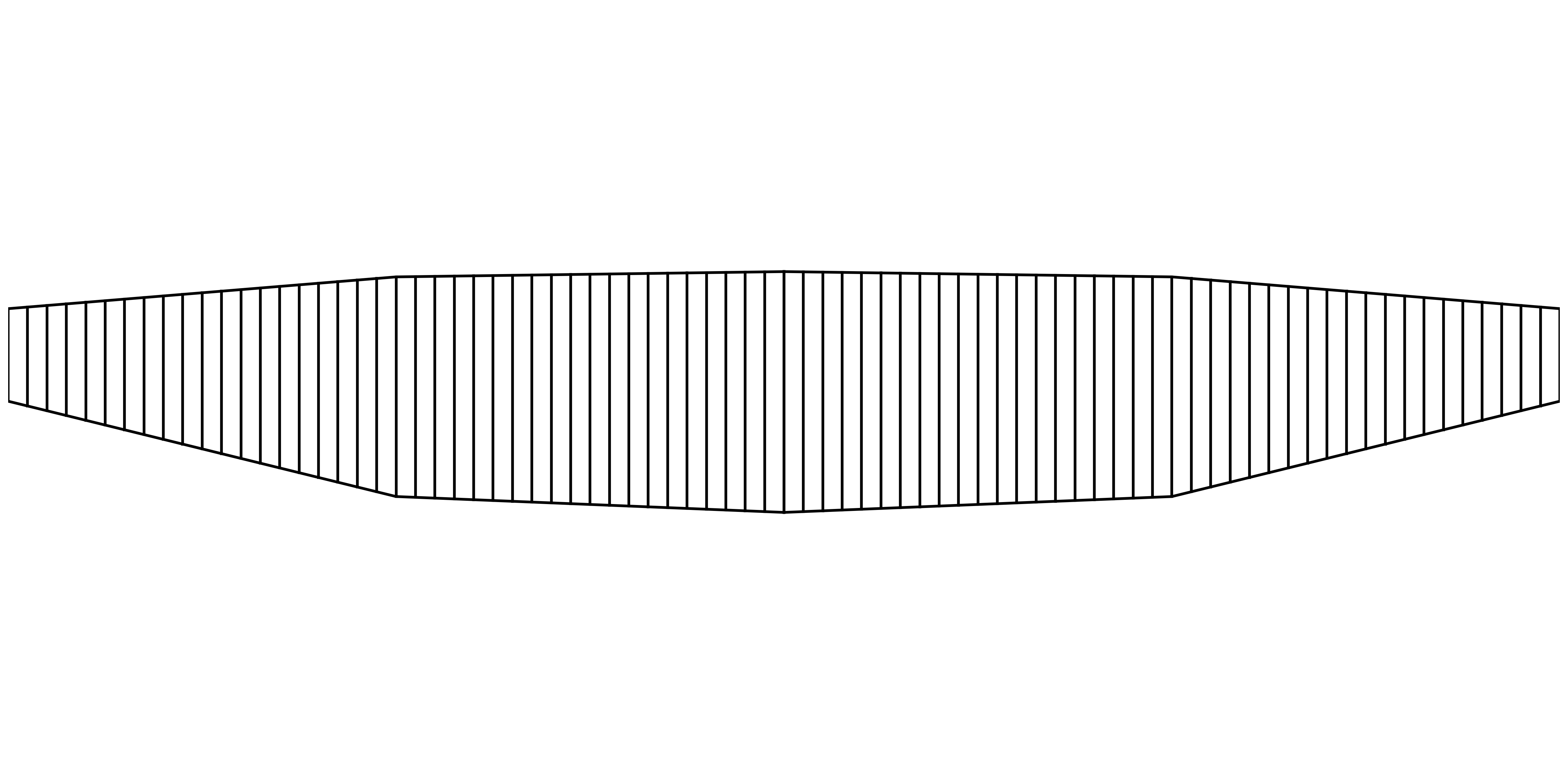
The following shows the resulting optimized mesh. The result is identical regardless of if the constraint-based or construction-based joining approahces are used.
Constraint-based Approach
Setting up the multi-section goemetry group with the constrint-based approach for section joining requires a slightly different inital setup. The constraint can be enforced at the leading and/or trailing edge of each segment junction in any combination of x, y, or z directions. A fully differentiated implementation that facilitates setting this constraint is incorporated into OAS. This approach is robust but introduces at least two linear constraints per segment junction. The steps required to setup the multi-section geometry group by constraint feature differences from the construction-based approach starting at the geometry group setup.
# Instead of creating a standard geometery group, here we will create a multi-section group that will accept our multi-section surface
# dictionary and allow us to specify any C0 continuity constraints between the sections. In this example we will constrain the sections
# into a C0 continuous surface using a component that the optimizer can use as a constraint. The joining constraint component returns the
# distance between the leading edge and trailing edge points at section interections. Any combination of the x,y, and z distances can be returned
# to constrain the surface in a particular direction.


"""
                        LE1              LE2   cLE = [LE2x-LE1x,LE2y-LE1y,LE2z-LE1z]
------------------------- <-------------> -------------------------
|                       |                 |                       |
|                       |                 |                       |
|        sec 0          |                 |         sec 1         |
|                       |                 |     "root section"    |
|______________________ | <-------------> |_______________________|
                        TE1              TE2    cTE = [TE2x-TE1x,TE2y-TE1y,TE2z-TE1z]


"""

# We pass in the multi-section surface dictionary to the MultiSecGeometry geometery group. We also enabled joining_comp and pass two array to dim_contr
# These two arrays should only consists of 1 and 0 and tell the joining component which of the x,y, and z distance constraints we wish to enforce at the LE and TE
# In this example, we only wish to constraint the x-distance between the sections at both the leading and trailing edge.

multi_geom_group = MultiSecGeometry(
    surface=surface, joining_comp=True, dim_constr=[np.array([1, 0, 0]), np.array([1, 0, 0])]
)
prob.model.add_subsystem(surface["name"], multi_geom_group)


# In this next part, we will setup the aerodynamics group. First we use a utility function called build_section_dicts which takes our multi-section surface dictionary and outputs a
# surface dictionary for each individual section. We then inputs these dictionaries into the mesh unification function unify_mesh to produce a single mesh array for the the entire surface.
# We then add this mesh to the multi-section surface dictionary
section_surfaces = build_section_dicts(surface)
uniMesh = unify_mesh(section_surfaces)
surface["mesh"] = uniMesh

# Create the aero point group, which contains the actual aerodynamic
# analyses. This step is exactly as it's normally done except the surface dictionary we pass in is the multi-surface one
aero_group = AeroPoint(surfaces=[surface])
point_name = "aero_point_0"
prob.model.add_subsystem(point_name, aero_group, promotes_inputs=["v", "alpha", "Mach_number", "re", "rho", "cg"])


# The following steps are similar to a normal OAS surface script but note the differences in surface naming. Note that
# unified surface created by the multi-section geometry group needs to be connected to AeroPoint(be careful with the naming)

# Get name of surface and construct the name of the unified surface mesh
name = surface["name"]
unification_name = "{}_unification".format(surface["name"])

# Connect the mesh from the mesh unification component to the analysis point.
prob.model.connect(name + "." + unification_name + "." + name + "_uni_mesh", point_name + "." + "surface" + ".def_mesh")

# Perform the connections with the modified names within the
# 'aero_states' group.
prob.model.connect(
    name + "." + unification_name + "." + name + "_uni_mesh", point_name + ".aero_states." + "surface" + "_def_mesh"
)


# Next, we add the DVs to the OpenMDAO problem. Note that each surface's geometeric parameters are under the given section names specified in the multi-surface dictionary earlier.
# Here we use the chord B-spline that we specified earlier for each section and the angle-of-attack as DVs.
prob.model.add_design_var("surface.sec0.chord_cp", lower=0.1, upper=10.0, units=None)
prob.model.add_design_var("surface.sec1.chord_cp", lower=0.1, upper=10.0, units=None)
prob.model.add_design_var("alpha", lower=0.0, upper=10.0, units="deg")


# Next, we add the C0 continuity constraint for this problem by constraining the x-distance between sections to 0.
# NOTE: SLSQP optimizer does not handle the joining equality constraint properly so the constraint needs to be specified as an inequality constraint
# All other optimizers like SNOPT can handle the equality constraint as is.

prob.model.add_constraint("surface.surface_joining.section_separation", upper=0, lower=0)  # FOR SLSQP
# prob.model.add_constraint('surface.surface_joining.section_separation',equals=0.0,scaler=1e-4) #FOR OTHER OPTIMIZERS

# Add CL constraint
prob.model.add_constraint(point_name + ".CL", equals=0.3)

# Add Wing total area constraint
prob.model.add_constraint(point_name + ".total_perf.S_ref_total", equals=2.0)

# Add objective
prob.model.add_objective(point_name + ".CD", scaler=1e4)


prob.driver = om.ScipyOptimizeDriver()
prob.driver.options["optimizer"] = "SLSQP"
prob.driver.options["tol"] = 1e-3
prob.driver.options["disp"] = True
prob.driver.options["maxiter"] = 1000

# Set up and run the optimization problem
prob.setup()
prob.run_driver()
# om.n2(prob)
Multi-section surfaces for aerostructural problems
Both multi-section geometery parameterization approaches in OpenAeroStruct are fully compatible with the aerostructural simulation capability through the multi-section aerostructural geometery class. Both the tube and wingbox models can be used however note that the structural model itself is not multi-section. The structural member geometery is not defined for each section but rather the entire surface as it normally is. The finite-element beam model is therefore coupled with the unified surface mesh which is where the aerodynamic simulation is done.
We start by making the necessary imports for an aerostructural optimization in OpenAeroStruct. Note that we also import a special geometry group for multi-section aerostructural problems.
import numpy as np
import openmdao.api as om
from openaerostruct.integration.aerostruct_groups import MultiSecAerostructGeometry, AerostructPoint
from openaerostruct.utils.constants import grav_constant
from openaerostruct.geometry.utils import build_section_dicts, unify_mesh, build_multi_spline, connect_multi_spline
Next, we define the surface dictionary as we did for the construction-based multi-section geometry parameterization but also include the structural parameters.
# The geometry parameterization used here is identical to the one in the two section contruction based example. However,
# instead of chord we apply the principle to the twist B-spline.

# Set-up B-splines for each section. Done here since this information will be needed multiple times.
sec_twist_cp = [np.zeros(2), np.zeros(2)]

# Note the additional of structural variables to the surface dictionary
surface = {
    # Wing definition
    # Basic surface parameters
    "name": "surface",
    "is_multi_section": True,
    "num_sections": 2,  # The number of sections in the multi-section surface
    "sec_name": ["sec0", "sec1"],  # names of the individual sections
    "symmetry": True,  # if true, model one half of wing. reflected across the midspan of the root section
    "S_ref_type": "wetted",  # how we compute the wing area, can be 'wetted' or 'projected'
    "root_section": 1,
    # Geometry Parameters
    "taper": [1.0, 1.0],  # Wing taper for each section
    "span": [10.0, 10.0],  # Wing span for each section
    "sweep": [0.0, 0.0],  # Wing sweep for each section
    "twist_cp": sec_twist_cp,
    "t_over_c_cp": [np.array([0.15]), np.array([0.15])],  # thickness over chord ratio (NACA0015)
    "root_chord": 5.0,  # Wing root chord for each section
    # Mesh Parameters
    "meshes": "gen-meshes",  # Supply a mesh for each section or "gen-meshes" for automatic mesh generation
    "nx": 2,  # Number of chordwise points. Same for all sections
    "ny": [3, 3],  # Number of spanwise points for each section
    # Aerodynamic Parameters
    "CL0": 0.0,  # CL of the surface at alpha=0
    "CD0": 0.015,  # CD of the surface at alpha=0
    # Airfoil properties for viscous drag calculation
    "k_lam": 0.05,  # percentage of chord with laminar
    # flow, used for viscous drag
    "c_max_t": 0.303,  # chordwise location of maximum (NACA0015)
    # thickness
    "with_viscous": True,  # if true, compute viscous drag
    "with_wave": False,  # if true, compute wave drag
    "groundplane": False,
    # Structural
    "fem_model_type": "tube",
    "thickness_cp": 0.1 * np.ones((2)),
    "E": 70.0e9,  # [Pa] Young's modulus of the spar
    "G": 30.0e9,  # [Pa] shear modulus of the spar
    "yield": 500.0e6 / 2.5,  # [Pa] yield stress divided by 2.5 for limiting case
    "mrho": 3.0e3,  # [kg/m^3] material density
    "fem_origin": 0.35,  # normalized chordwise location of the spar
    "wing_weight_ratio": 2.0,
    "struct_weight_relief": False,  # True to add the weight of the structure to the loads on the structure
    "distributed_fuel_weight": False,
    # Constraints
    "exact_failure_constraint": False,  # if false, use KS function
}
The independent variables and unified twist spline are setup in the same way as in the construction-based multi-section geometry parameterization.
# Create the problem and assign the model group
prob = om.Problem(reports=False)

# Add problem information as an independent variables component
indep_var_comp = om.IndepVarComp()
indep_var_comp.add_output("v", val=248.136, units="m/s")
indep_var_comp.add_output("alpha", val=9.0, units="deg")
indep_var_comp.add_output("Mach_number", val=0.84)
indep_var_comp.add_output("re", val=1.0e6, units="1/m")
indep_var_comp.add_output("rho", val=0.38, units="kg/m**3")
indep_var_comp.add_output("CT", val=grav_constant * 17.0e-6, units="1/s")
indep_var_comp.add_output("R", val=11.165e6, units="m")
indep_var_comp.add_output("W0", val=0.4 * 3e5, units="kg")
indep_var_comp.add_output("speed_of_sound", val=295.4, units="m/s")
indep_var_comp.add_output("load_factor", val=1.0)
indep_var_comp.add_output("empty_cg", val=np.zeros((3)), units="m")

prob.model.add_subsystem("prob_vars", indep_var_comp, promotes=["*"])


# Generate the sections and unified mesh here in addition to adding the components.
# This has to also be done here since AeroPoint has to know the unified mesh size.
section_surfaces = build_section_dicts(surface)
uniMesh = unify_mesh(section_surfaces)
surface["mesh"] = uniMesh


# Build a component with B-spline control points that joins the sections by construction
twist_comp = build_multi_spline("twist_cp", len(section_surfaces), sec_twist_cp)
prob.model.add_subsystem("twist_bspline", twist_comp)

# Connect the B-spline component to the section B-splines
connect_multi_spline(prob, section_surfaces, sec_twist_cp, "twist_cp", "twist_bspline", surface["name"])
Next, we add the multi-section aerostructural geometery and aerostructural analysis point groups and make the necessary connections. Note that this step is very similar to the single section aerostructural problem setup with only the geometery group being replaced.
# Create and add a group that handles the geometry for the
# aerostructual multi-section lifting surface
multi_geom_group = MultiSecAerostructGeometry(surface=surface)
prob.model.add_subsystem(surface["name"], multi_geom_group)

name = surface["name"]

point_name = "AS_point_0"

# Create the aero point group and add it to the model
AS_point = AerostructPoint(surfaces=[surface])

prob.model.add_subsystem(
    point_name,
    AS_point,
    promotes_inputs=[
        "v",
        "alpha",
        "Mach_number",
        "re",
        "rho",
        "CT",
        "R",
        "W0",
        "speed_of_sound",
        "empty_cg",
        "load_factor",
    ],
)

com_name = point_name + "." + name + "_perf"
prob.model.connect(name + ".local_stiff_transformed", point_name + ".coupled." + name + ".local_stiff_transformed")
prob.model.connect(name + ".nodes", point_name + ".coupled." + name + ".nodes")

# Connect aerodyamic mesh to coupled group mesh
prob.model.connect(name + ".mesh", point_name + ".coupled." + name + ".mesh")

# Connect performance calculation variables
prob.model.connect(name + ".radius", com_name + ".radius")
prob.model.connect(name + ".thickness", com_name + ".thickness")
prob.model.connect(name + ".nodes", com_name + ".nodes")
prob.model.connect(name + ".cg_location", point_name + "." + "total_perf." + name + "_cg_location")
prob.model.connect(name + ".structural_mass", point_name + "." + "total_perf." + name + "_structural_mass")
prob.model.connect(name + ".t_over_c", com_name + ".t_over_c")
We can now setup our optimization problem, configure the optimizer and run the optimization.
prob.driver = om.ScipyOptimizeDriver()
prob.driver.options["optimizer"] = "SLSQP"
prob.driver.options["tol"] = 1e-6
prob.driver.options["disp"] = True
prob.driver.options["maxiter"] = 1000


# Setup problem and add design variables, constraint, and objective
prob.model.add_design_var("twist_bspline.twist_cp_spline", lower=-10.0, upper=15.0)
prob.model.add_design_var("surface.thickness_cp", lower=0.01, upper=0.5, scaler=1e2)
prob.model.add_constraint("AS_point_0.surface_perf.failure", upper=0.0)
prob.model.add_constraint("AS_point_0.surface_perf.thickness_intersects", upper=0.0)

# Add design variables, constraints, and objective on the problem
prob.model.add_design_var("alpha", lower=-10.0, upper=10.0)
prob.model.add_constraint("AS_point_0.L_equals_W", equals=0.0)
prob.model.add_objective("AS_point_0.fuelburn", scaler=1e-5)


# Set up the problem
prob.setup(check=True)

# Run the optimization
optResult = prob.run_driver()
# om.n2(prob, show_browser=False)
Lastly, we plot and print the results.
# Print fuelburn
print(prob.get_val("AS_point_0.fuelburn"))