Aerodynamic Optimization

This page documents in detail how we perform aerodynamic optimization in OpenAeroStruct. You should read this page in its entirety to get a feel for how the model is set up and used.

OpenMDAO basics

OpenAeroStruct is a tool written using the OpenMDAO framework. OpenMDAO is an open-source high-performance computing platform for systems analysis and multidisciplinary optimization, written in Python. Visit OpenMDAO’s documentation for information on its capabilities and API.

Here is an extremely quick rundown of the basic terminology within OpenMDAO:

Component: smallest unit of computational work
Group: container used to build up model hierarchies
Driver: controls iterative model execution process (e.g., Optimizer, DOE)
Problem: top level class that contains everything and provide the model execution API

Intro to the structure of the OpenAeroStruct problem

In general, you’ll follow these four steps to set up and run a problem in OpenAeroStruct:

Define your lifting surface
Initialize your problem and add flow conditions
Add your design variables, constraints, and objective
Set up and run the optimization problem

We’ll now investigate these steps individually using an aerodynamic optimization case as an example. The full run script for this case is in Quick Example.

1. Define your lifting surface

In the simplest case, you can add a single lifting surface that represents the wing of an aircraft. To define a lifting surface, you first need to produce a computational mesh that represents that surface.

OpenAeroStruct contains a helper function to create these meshes or you can create your own array of points through another method. To use OpenAeroStruct’s helper function, you need to give it the number of spanwise points, num_y, the number of chordwise points, num_x, and the type of baseline planform to start with, wing_type. There are two main options for wing_type: rect, which is a rectangular wing, and CRM, which is based on the Common Research Model wing. This example uses the CRM option. See the run_scaneagle.py example in the examples/ directory for an example that uses the rect option. The rect option is convenient for simple rectangular and trapezoidal planforms. Alternatively, if you want to create your own custom mesh, see Multi-section Surfaces.

In the code block shown below, we call the helper function to define a mesh and get a starting twist distribution.

import numpy as np

import openmdao.api as om

from openaerostruct.geometry.utils import generate_mesh
from openaerostruct.geometry.geometry_group import Geometry
from openaerostruct.aerodynamics.aero_groups import AeroPoint

# Create a dictionary to store options about the mesh
mesh_dict = {"num_y": 7, "num_x": 2, "wing_type": "CRM", "symmetry": True, "num_twist_cp": 5}

# Generate the aerodynamic mesh based on the previous dictionary
mesh, twist_cp = generate_mesh(mesh_dict)

There are many options for each surface, and they are loosely organized into the following categories:

Wing definition (mesh, wing position, symmetry option, etc)
Geometric variable definitions (span, dihedral, sweep, twist, etc)
Aerodynamic performance (CL and CD at angle of attack=0)
Airfoil properties (turbulence transition point, t/c, location of max t)
Structural properties (E, G, yield stress, location of spar, etc)
Options for constraints (KS aggregation, monotonic design variables)

# Create a dictionary with info and options about the aerodynamic
# lifting surface
surface = {
    # Wing definition
    "name": "wing",  # name of the surface
    "symmetry": True,  # if true, model one half of wing
    # reflected across the plane y = 0
    "S_ref_type": "wetted",  # how we compute the wing area,
    # can be 'wetted' or 'projected'
    "fem_model_type": "tube",
    "twist_cp": twist_cp,
    "mesh": mesh,
    # Aerodynamic performance of the lifting surface at
    # an angle of attack of 0 (alpha=0).
    # These CL0 and CD0 values are added to the CL and CD
    # obtained from aerodynamic analysis of the surface to get
    # the total CL and CD.
    # These CL0 and CD0 values do not vary wrt alpha.
    "CL0": 0.0,  # CL of the surface at alpha=0
    "CD0": 0.015,  # CD of the surface at alpha=0
    # Airfoil properties for viscous drag calculation
    "k_lam": 0.05,  # percentage of chord with laminar
    # flow, used for viscous drag
    "t_over_c_cp": np.array([0.15]),  # thickness over chord ratio (NACA0015)
    "c_max_t": 0.303,  # chordwise location of maximum (NACA0015)
    # thickness
    "with_viscous": True,  # if true, compute viscous drag
    "with_wave": False,  # if true, compute wave drag
}

For more details about mesh_dict and surface, see Mesh and Surface Dictionaries.

2. Initialize your problem and add problem conditions

Next, we need to initialize the OpenMDAO problem, add flow conditions, and add the groups that contain the analysis components. In a more complex model, these flow conditions might come from a different OpenMDAO component, but here we hook them up into the model using an independent variable component, or IndepVarComp. Set the values for these parameters that you want to use here. We then add this component to the OpenMDAO model.

# Create the OpenMDAO problem
prob = om.Problem()

# Create an independent variable component that will supply the flow
# conditions to the problem.
indep_var_comp = om.IndepVarComp()
indep_var_comp.add_output("v", val=248.136, units="m/s")
indep_var_comp.add_output("alpha", val=5.0, units="deg")
indep_var_comp.add_output("Mach_number", val=0.84)
indep_var_comp.add_output("re", val=1.0e6, units="1/m")
indep_var_comp.add_output("rho", val=0.38, units="kg/m**3")
indep_var_comp.add_output("cg", val=np.zeros((3)), units="m")

# Add this IndepVarComp to the problem model
prob.model.add_subsystem("prob_vars", indep_var_comp, promotes=["*"])

We now need to provide the geometry and analysis groups to the OpenMDAO problem.

We instantiate and add the Geometry group, which computes the new mesh shape based on the current values of the design parameters. In an optimization context, the driver will change these values, and the geometry group computes the new mesh to use in the analysis components.

We then add an AeroPoint group, which contains the analysis components to compute the aerodynamic performance of the lifting surface. Additionally, we promote the flow condition variables from the group up to the model level. This means that the values in our IndepVarComp can pass data into this AeroPoint group, which is how the aerodynamic analysis knows which flow conditions to use.

We need to connect some of the variables from the Geometry group into the AeroPoint group. These connections allow information about the mesh to flow through the model correctly.

# Create and add a group that handles the geometry for the
# aerodynamic lifting surface
geom_group = Geometry(surface=surface)
prob.model.add_subsystem(surface["name"], geom_group)

# Create the aero point group, which contains the actual aerodynamic
# analyses
aero_group = AeroPoint(surfaces=[surface])
point_name = "aero_point_0"
prob.model.add_subsystem(point_name, aero_group, promotes_inputs=["v", "alpha", "Mach_number", "re", "rho", "cg"])

name = surface["name"]

# Connect the mesh from the geometry component to the analysis point
prob.model.connect(name + ".mesh", point_name + "." + name + ".def_mesh")

# Perform the connections with the modified names within the
# 'aero_states' group.
prob.model.connect(name + ".mesh", point_name + ".aero_states." + name + "_def_mesh")

prob.model.connect(name + ".t_over_c", point_name + "." + name + "_perf." + "t_over_c")

3. Add your design variables, constraints, and objective

Note

This step is only necessary when performing an optimization and is not needed for only analysis.

With the problem and surfaces defined, we can now add a description of the optimization problem.

You can use a certain set of parameters as design variables, including:

angle of attack
taper
span
dihedral
sweep
chord distribution
twist distribution
shear deformation in x direction
shear deformation in y direction
structural spar radius distribution
structural spar thickness distribution

For the constraints and objective, you can use any outputted variable. Common constraints include:

structural failure
CL = fixed value
monotonic constraint on spanwise variable (e.g. chord can only get decrease as you go outboard)

Common objectives include:

weight
fuel burn
CL
CD

We also tell the OpenMDAO problem to record information about each optimization iteration. This will allow us to visualize the history during and after the optimization.

# Import the Scipy Optimizer and set the driver of the problem to use
# it, which defaults to an SLSQP optimization method
import openmdao.api as om

prob.driver = om.ScipyOptimizeDriver()
prob.driver.options["tol"] = 1e-9

recorder = om.SqliteRecorder("aero_analysis_test.db")
prob.driver.add_recorder(recorder)
prob.driver.recording_options["record_derivatives"] = True
prob.driver.recording_options["includes"] = ["*"]

# Setup problem and add design variables, constraint, and objective
prob.model.add_design_var("wing.twist_cp", lower=-10.0, upper=15.0)
prob.model.add_constraint(point_name + ".wing_perf.CL", equals=0.5)
prob.model.add_objective(point_name + ".wing_perf.CD", scaler=1e4)

1. Set up and run the optimization problem

With the problem defined, we can now actually run the optimization. If you only wanted to perform analysis, not optimization, you could use prob.run_model() instead of prob.run_driver() in the code below.

The code below find the lowest CD value while providing a certain amount of lift by constraining CL.

# Set up and run the optimization problem
prob.setup()
prob.run_driver()

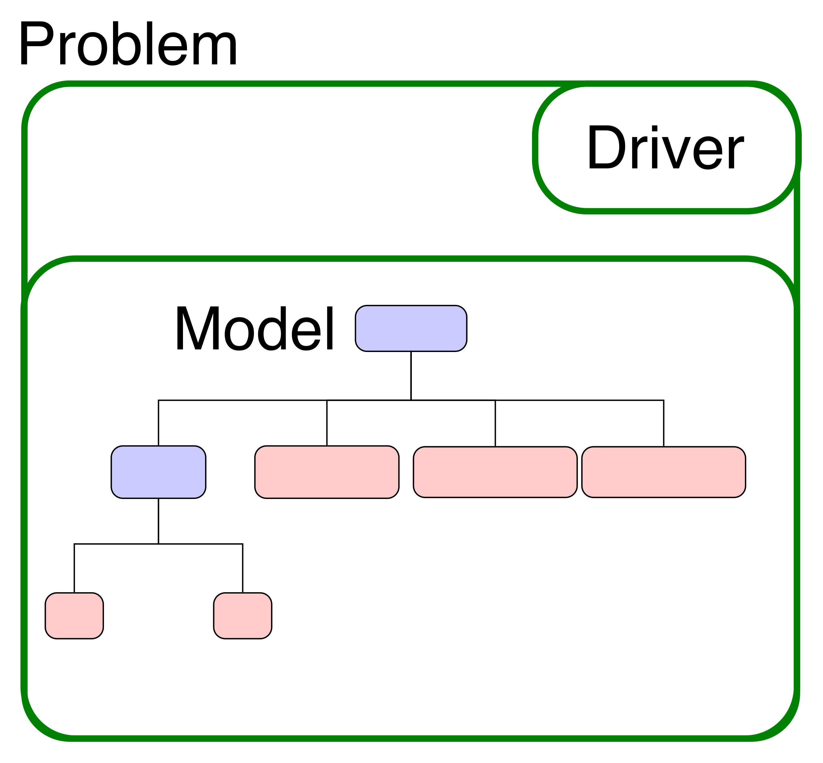
Investigation of the problem structure – N2 diagram

We’ll now take a moment to explain the organization of the aerodynamic model.

Mouse over components and parameters to see the data-passing connections between them. You can expand this view, click on boxes to zoom in, or right-click to collapse boxes. This shows the layout of the components within the OpenAeroStruct model. There’s also a help button (the ? mark) on the far right of the top toolbar with information about more features.

To create this diagram for any OpenMDAO problem, add these two lines after you call prob.setup():

from openmdao.api import n2
n2(prob)

Use any web browser to open the .html file and you can examine your problem layout. This diagram shows groups in dark blue, components in light blue, as organized by your actual problem hierarchy. Parameters (inputs and outputs) are shown on the diagonal, with off-diagonal terms representing where an output from a component is passed as input to another component. Any red parameters shown are unconnected inputs, which means that those parameters are not receiving any data from another component. In general this is bad – it suggests that the model is not set up properly – but if you want to use the default value of those inputs, then it’s OK. For example, we currently have unconnected inputs in the geometry group within OpenAeroStruct, but this is allowable because the default values used in that group are correct and do not modify the mesh.

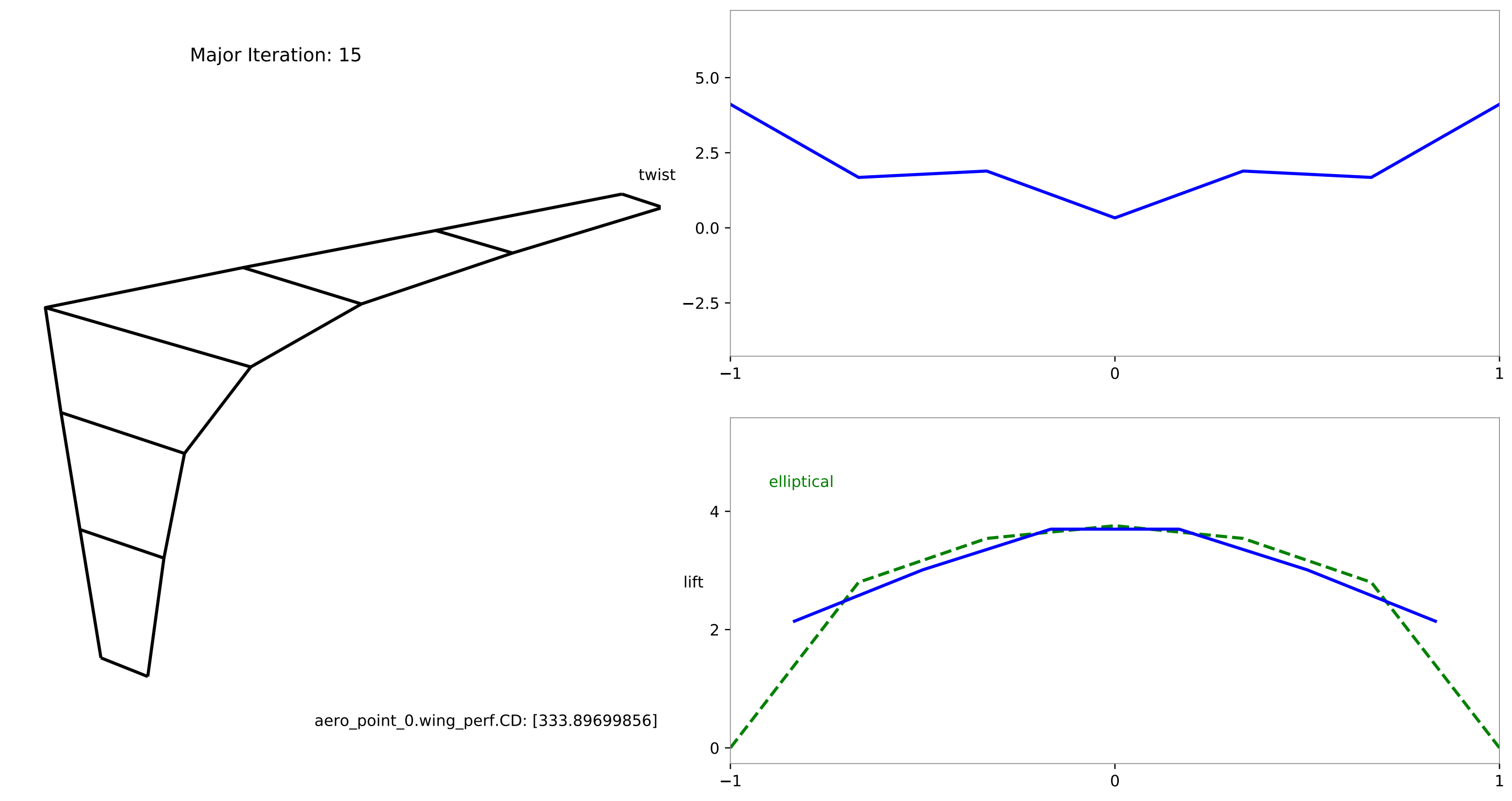
How to visualize results

You can visualize the lifting surface and structural spar using:

plot_wing aero.db

Here you’ll use aero.db or the filename for where you saved the problem data. This will produce a window where you can see how the lifting surface and design variables change with each iteration, as shown below. You can monitor the results from your optimization as it progresses by checking the Automatically refresh button.