Aerostructural Optimization with Wingbox
In addition to the tubular-spar structural model available in OpenAeroStruct, you can use a wingbox-based model. This model is described in Chauhan and Martins’ paper here. We strongly recommend reading this relatively short conference paper to learn about the model and see some example results. The presentation slides for this conference paper can be found online. Analytic derivatives are not provided for some components of this model, so any optimization problem will use the complex-step approximation to obtain the relevant partial derivatives for these components.
This page breaks down and describes an example optimization run-script that uses the wingbox model. This example uses the same optimization problem used for the paper linked above, but with fewer design variables and a coarser mesh. The wing being optimized is based on the undeflected Common Research Model (uCRM), which is a long-range transport aircraft. A script to replicate the optimization problems described in the paper can be found in the examples directory (openaerostruct/examples/run_aerostruct_uCRM_multipoint.py).
The goal of the wingbox model is to allow more realistic preliminary structural sizing for commuter to long-range transport-type aircraft which typically have wingbox structures. Since more realistic sizing is one of the goals of the wingbox model, this example also shows how to use it with a multipoint optimization. Wing structures are usually sized using loads that do not occur during normal cruise conditions, so we must consider at least one more flight point that provides more extreme loads.
This tutorial assumes that the reader has gone through the other examples and tutorials in the OpenAeroStruct documentation and is now familiar with how to set up problems and the terminology of OpenAeroStruct.
Let’s begin and look at the run-script now. First we import some modules.
import numpy as np
from openaerostruct.meshing.mesh_generator import generate_mesh
from openaerostruct.integration.aerostruct_groups import AerostructGeometry, AerostructPoint
from openaerostruct.structures.wingbox_fuel_vol_delta import WingboxFuelVolDelta
import openmdao.api as om
Next, we provide some airfoil coordinates. These coordinates are used to define the shape of the wingbox cross-section. In this example, we use the NASA SC2-0612 coordinates from airfoiltools.com. However, here we only provide the coordinates for the 10%- to 60%-chord portion of the airfoil because for this example we assume that it is this portion of the chord along the wing that will be structural and form the wingbox. Make sure that the first and last x-coordinates (chordwise) of the upper and lower curves are the same. Also make sure that the chord length of the original airfoil has been normalized to 1 (this is normally the case for the airfoil coordinates available on airfoiltools.com).
These coordinates will be scaled based on the effective chord and thickness-to-chord ratio for each wingbox segment along the wing. However, we currently have not implemented the functionality to specify different airfoil coordinates for different segments of the wing, so the same coordinates are used for the entire wing.
# Provide coordinates for a portion of an airfoil for the wingbox cross-section as an nparray with dtype=complex (to work with the complex-step approximation for derivatives).
# These should be for an airfoil with the chord scaled to 1.
# We use the 10% to 60% portion of the NASA SC2-0612 airfoil for this case
# We use the coordinates available from airfoiltools.com. Using such a large number of coordinates is not necessary.
# The first and last x-coordinates of the upper and lower surfaces must be the same

# fmt: off
upper_x = np.array([0.1, 0.11, 0.12, 0.13, 0.14, 0.15, 0.16, 0.17, 0.18, 0.19, 0.2, 0.21, 0.22, 0.23, 0.24, 0.25, 0.26, 0.27, 0.28, 0.29, 0.3, 0.31, 0.32, 0.33, 0.34, 0.35, 0.36, 0.37, 0.38, 0.39, 0.4, 0.41, 0.42, 0.43, 0.44, 0.45, 0.46, 0.47, 0.48, 0.49, 0.5, 0.51, 0.52, 0.53, 0.54, 0.55, 0.56, 0.57, 0.58, 0.59, 0.6], dtype="complex128")
lower_x = np.array([0.1, 0.11, 0.12, 0.13, 0.14, 0.15, 0.16, 0.17, 0.18, 0.19, 0.2, 0.21, 0.22, 0.23, 0.24, 0.25, 0.26, 0.27, 0.28, 0.29, 0.3, 0.31, 0.32, 0.33, 0.34, 0.35, 0.36, 0.37, 0.38, 0.39, 0.4, 0.41, 0.42, 0.43, 0.44, 0.45, 0.46, 0.47, 0.48, 0.49, 0.5, 0.51, 0.52, 0.53, 0.54, 0.55, 0.56, 0.57, 0.58, 0.59, 0.6], dtype="complex128")
upper_y = np.array([ 0.0447,  0.046,  0.0472,  0.0484,  0.0495,  0.0505,  0.0514,  0.0523,  0.0531,  0.0538, 0.0545,  0.0551,  0.0557, 0.0563,  0.0568, 0.0573,  0.0577,  0.0581,  0.0585,  0.0588,  0.0591,  0.0593,  0.0595,  0.0597,  0.0599,  0.06,    0.0601,  0.0602,  0.0602,  0.0602,  0.0602,  0.0602,  0.0601,  0.06,    0.0599,  0.0598,  0.0596,  0.0594,  0.0592,  0.0589,  0.0586,  0.0583,  0.058,   0.0576,  0.0572,  0.0568,  0.0563,  0.0558,  0.0553,  0.0547,  0.0541], dtype="complex128")  # noqa: E201, E241
lower_y = np.array([-0.0447, -0.046, -0.0473, -0.0485, -0.0496, -0.0506, -0.0515, -0.0524, -0.0532, -0.054, -0.0547, -0.0554, -0.056, -0.0565, -0.057, -0.0575, -0.0579, -0.0583, -0.0586, -0.0589, -0.0592, -0.0594, -0.0595, -0.0596, -0.0597, -0.0598, -0.0598, -0.0598, -0.0598, -0.0597, -0.0596, -0.0594, -0.0592, -0.0589, -0.0586, -0.0582, -0.0578, -0.0573, -0.0567, -0.0561, -0.0554, -0.0546, -0.0538, -0.0529, -0.0519, -0.0509, -0.0497, -0.0485, -0.0472, -0.0458, -0.0444], dtype="complex128")
# fmt: on
Next, we create the dictionary with information for the mesh and create the mesh. For this example we use the uCRM-based geometry (undeflected Common Research Model) already defined and available in OpenAeroStruct. Alternatively, the user can provide their own mesh (see Multi-section surfaces for aerodynamic problems for another example with a custom mesh). Here we specify 15 as the number of spanwise nodes and 3 as the number of chordwise nodes for the VLM mesh. We also set chord_cos_spacing and span_cos_spacing to 0 for uniform panel spacing. The FEM model will use the spanwise spacing of the VLM mesh for the FEM mesh. We use a very coarse mesh for this example to keep the computational time low.
The generate_mesh function takes the inputs from the mesh dictionary and returns the mesh as well as values for the B-spline control points for the twist distribution (we specify the number of control points for this using num_twist_cp in the dictionary). Note that in this example we don’t end up using this twist distribution, but instead use a better starting twist distribution which will be seen later.
# Create a dictionary to store options about the surface
mesh_dict = {
    "num_y": 15,
    "num_x": 3,
    "wing_type": "uCRM_based",
    "symmetry": True,
    "chord_cos_spacing": 0,
    "span_cos_spacing": 0,
    "num_twist_cp": 4,
}

mesh, twist_cp = generate_mesh(mesh_dict)
Next, we create a surface dictionary and provide necessary information for our lifting surface. After providing the relevant information for the name, symmetry, and S_ref_type settings, we provide the mesh and specify the string ‘wingbox’ for the fem_model_type (if we wanted the tubular structure, we would specify ‘tube’ instead). We also provide the airfoil coordinates for the wingbox cross-section here as the four arrays defined earlier.
surf_dict = {
    # Wing definition
    "name": "wing",  # give the surface some name
    "symmetry": True,  # if True, model only one half of the lifting surface
    "S_ref_type": "projected",  # how we compute the wing area,
    # can be 'wetted' or 'projected'
    "mesh": mesh,
    "fem_model_type": "wingbox",  # 'wingbox' or 'tube'
    "data_x_upper": upper_x,
    "data_x_lower": lower_x,
    "data_y_upper": upper_y,
    "data_y_lower": lower_y,
Next, we provide some initial values for the wingbox spar and skin thickness distributions (B-spline control points), along with the wing twist distribution (note that these distributions do not need to have the same number of control points). For the wingbox model, to maintain simplicity, we use the same thickness variables for both the top and bottom wing skins. Similarly, we use the same thickness variables for the front and rear spars. Currently, we do not model buckling or have any buckling constraints. However, a comparison of optimized skin thicknesses with high-fidelity results shown in these slides, indicates that, assuming the wing has a reasonable rib spacing, this is not a very major concern.
We also provide a distribution for the thickness-to-chord ratio (B-spline control points for t_over_c_cp). The thickness-to-chord ratio design variable is important for the trade-off between aerodynamic (wave and viscous drag) benefits from a thin wing and structural benefits from a thick wing. The original_wingbox_airfoil_t_over_c is the thickness-to-chord ratio of the airfoil provided for the wingbox cross-section. For this example, the thickness-to-chord ratio of the SC2-0612 is 12%. This is used to scale the airfoil in the thickness direction as the thickness-to-chord ratio variable changes. Note that the thickness-to-chord ratio variable is the streamwise value. Using the sweep angle for the wingbox elements OpenAeroStruct computes the effective values for the wingbox cross-sections normal to the elements.
    "twist_cp": np.array([4.0, 5.0, 8.0, 9.0]),  # [deg]
    "spar_thickness_cp": np.array([0.004, 0.005, 0.008, 0.01]),  # [m]
    "skin_thickness_cp": np.array([0.005, 0.01, 0.015, 0.025]),  # [m]
    "t_over_c_cp": np.array([0.08, 0.08, 0.10, 0.08]),
    "original_wingbox_airfoil_t_over_c": 0.12,
Next, we provide some information related to aerodynamics and specify some options. We set CDO to 0.0078 to account for the drag from the fuselage, tail surfaces, nacelles, and pylons (which are not being modeled). We set with_viscous to True to make OpenAeroStruct include an estimate for viscous drag (empirical equations) when computing the drag of the wing. We set with_wave to True to make OpenAeroStruct also include an estimate for wave drag using the empirical equations based on the Korn equation. This wave drag estimate needs a thickness-to-chord ratio value and a sweep angle value for the wing. This is computed internally by averaging the thickness-to-chord ratios and sweep angles across the span of the wing weighted by the widths of the corresponding VLM panels. Keep this in mind when creating wing meshes and setting up optimization problems using the wingbox model. The optimizer may try to take advantage of this averaging.
The k_lam value is the fraction of the chord assumed to have laminar flow, and is used for OpenAeroStruct’s viscous drag estimates (empirical equations). The c_max_t value is the location of the maximum thickness of the airfoil along the chord, and is also used for OpenAeroStruct’s viscous drag estimates.
    # Aerodynamic deltas.
    # These CL0 and CD0 values are added to the CL and CD
    # obtained from aerodynamic analysis of the surface to get
    # the total CL and CD.
    # These CL0 and CD0 values do not vary wrt alpha.
    # They can be used to account for things that are not included, such as contributions from the fuselage, camber, etc.
    "CL0": 0.0,  # CL delta
    "CD0": 0.0078,  # CD delta
    "with_viscous": True,  # if true, compute viscous drag
    "with_wave": True,  # if true, compute wave drag
    # Airfoil properties for viscous drag calculation
    "k_lam": 0.05,  # fraction of chord with laminar
    # flow, used for viscous drag
    "c_max_t": 0.38,  # chordwise location of maximum thickness
Next we provide some information related to structures. We provide the Young’s and shear moduli, as well as the maximum yield stress and density of the material being used. The material can either be assumed to be isotropic (like aluminum) or orthotropic (like carbon fiber reinforced polymer). Here we use include a safety factor of 1.5 using the safety_factor key. The strength_factor_for_upper_skin value can be used to adjust the yield strength of the upper skin relative to the lower skin. For example, if we were using different alloys for the top and bottom skin (e.g., Al7075 vs Al2024) we would provide the maximum yield stress of the lower skin for yield and the ratio of the yield strengths of the upper skin to the lower skin for strength_factor_for_upper_skin. The wing_weight_ratio number is used to estimate the weight of other components not modeled in the wingbox structure (e.g., overlaps, fasteners, etc.). With the exact_failure_constraint set to False, we aggregate the stress constraints for the FEM elements into a single constraint using the Kreisselmeier–Steinhauser function. This helps reduce computational cost during optimization by replacing a large number of constraints (one for each stress combination for each element) with a single constraint.
    # Structural values are based on aluminum 7075
    "E": 73.1e9,  # [Pa] Young's modulus
    "G": (73.1e9 / 2 / 1.33),  # [Pa] shear modulus (calculated using E and the Poisson's ratio here)
    "yield": 420.0e6,  # [Pa] yield stress
    "safety_factor": 1.5,  # safety factor
    "mrho": 2.78e3,  # [kg/m^3] material density
    "strength_factor_for_upper_skin": 1.0,  # the yield stress is multiplied by this factor for the upper skin
    "wing_weight_ratio": 1.25,
    "exact_failure_constraint": False,  # if false, use KS function
The next two options struct_weight_relief and distributed_fuel_weight are used to specify whether the user wants the loads from the weight of the wingbox structure and the weight of the fuel to be distributed on the wing structure to provide load relief. The struct_weight_relief is for the loads from the weight of the structure (including the wing_weight_ratio factor). The distributed_fuel_weight is for the loads from the weight of the fuel, which is assumed to be distributed across the entire wing (the fraction of the total fuel that each wingbox segment, corresponding to each finite element, holds is equal to the ratio of its enclosed volume to the total enclosed volume of all the wingbox segments). We can also use the option n_point_masses if we want to add loads from point masses on to the wing structure (e.g., for engines). Here we set n_point_masses to 1 because we have one engine on each side of the aircraft (recall that we are using symmetry). If we did not want to add point masses, we would omit this option (do not set it to 0).
    "struct_weight_relief": True,
    "distributed_fuel_weight": True,
    "n_point_masses": 1,  # number of point masses in the system; in this case, the engine (omit option if no point masses)
Next, we specify the density of the fuel (used to compute fuel volume from fuel mass) and also specify how much fuel we are carrying as reserves. This reserve fuel weight is added to the weight of the aircraft for performance calculations as well as computing the loads from the fuel on the wing when using the distributed_fuel_weight option. With these two final options, we are done with the surface dictionary and add it to a list called surfaces (here we only have one surface, but in general we might have multiple). Documentation on the surface dictionary can also be found in Mesh and Surface Dictionaries.
    "fuel_density": 803.0,  # [kg/m^3] fuel density (only needed if the fuel-in-wing volume constraint is used)
    "Wf_reserve": 15000.0,  # [kg] reserve fuel mass
}

surfaces = [surf_dict]
Next, we instantiate the OpenMDAO Problem and specify the independent variables. We will use some of these variables later as design variables and some simply as inputs. First we provide some inputs related to the flight conditions (Mach number, airspeed, Reynolds number per unit length, air density, and speed of sound). Since we want to consider two flight points in this example (a nominal cruise case and a 2.5g maneuver case), we provide two values for each input that is different for the two cases. For example, our cruise Mach number is 0.85 and our maneuver Mach number is 0.64.
# Create the problem and assign the model group
prob = om.Problem()

# Add problem information as an independent variables component
indep_var_comp = om.IndepVarComp()
indep_var_comp.add_output("Mach_number", val=np.array([0.85, 0.64]))
indep_var_comp.add_output("v", val=np.array([0.85 * 295.07, 0.64 * 340.294]), units="m/s")
indep_var_comp.add_output(
    "re",
    val=np.array([0.348 * 295.07 * 0.85 * 1.0 / (1.43 * 1e-5), 1.225 * 340.294 * 0.64 * 1.0 / (1.81206 * 1e-5)]),
    units="1/m",
)
indep_var_comp.add_output("rho", val=np.array([0.348, 1.225]), units="kg/m**3")
indep_var_comp.add_output("speed_of_sound", val=np.array([295.07, 340.294]), units="m/s")
The following are some more independent variables. We have the thrust-specific fuel consumption, CT, cruise range, R, and the weight of the aircraft without the fuel required for the cruise point and without the weight of the wing structure and point masses, W0_without_point_masses. Since we are not interested in the fuel burn or range at the maneuver point, we only provide a single value for these inputs that will be used for the cruise fuel burn. Note that W0_without_point_masses includes the reserve fuel weight, which is why it is added here.
indep_var_comp.add_output("CT", val=0.53 / 3600, units="1/s")
indep_var_comp.add_output("R", val=14.307e6, units="m")
indep_var_comp.add_output("W0_without_point_masses", val=128000 + surf_dict["Wf_reserve"], units="kg")
Next, we specify the load factor for each flight point (1g for cruise and 2.5g for the maneuver case). We also provide values for the angle of attack. In this case, instead of providing two values as an array for one variable, we add two separate variables with different names (alpha and alpha_maneuver). We create two variables just for convenience because, for this example, we allow the optimizer to trim the aircraft for the maneuver case using the angle of attack for that flight point (by making it a design variable), but keep the angle of attack fixed for the cruise case and make the optimizer trim the aircraft for the cruise flight point using the twist distribution. We also include the empty center of gravity location here as a reminder that we could use it later for studies in which we include tail surfaces and consider pitching moments (not done in this example).
indep_var_comp.add_output("load_factor", val=np.array([1.0, 2.5]))
indep_var_comp.add_output("alpha", val=0.0, units="deg")
indep_var_comp.add_output("alpha_maneuver", val=0.0, units="deg")

indep_var_comp.add_output("empty_cg", val=np.zeros((3)), units="m")
Finally, we also add the fuel mass as an independent variable to use it as a design variable. This may seem like a strange design variable to have, but we do this from an optimization architecture point of view. Instead of directly transferring the fuel burn value from the cruise point to the maneuver point (used to calculate MTOW for the maneuver point), we instead create a constraint (shown later) and make the optimizer ensure that the value being used for the fuel mass is the same value that is computed in the cruise point. This also allows the flexibility to later decide that you want to use a different value for the fuel mass for the maneuver case (or any other flight point you may have) that does not depend on the cruise point (or any other flight point you may have).
indep_var_comp.add_output("fuel_mass", val=10000.0, units="kg")

prob.model.add_subsystem("prob_vars", indep_var_comp, promotes=["*"])
Next, we include the engine mass magnitude and locations in the problem. OpenAeroStruct can handle any generic point masses add to the structural system. In this case, we’re adding the engine mass, which is set to 10,000 kg, to an appropriate location in front of the wing. The point_mass_locations coordinates are in the global frame. The loads caused by the point masses are transferred to the structural nodes based on the nodes’ proximity to the point masses (using an inverse-distance approach). We then compute the actual W0 value by summing the point_masses and W0_without_point_masses. We multiply the sum of point_masses by 2 because we are using symmetry. Thus, the W0 value used in subsequent components includes the point masses, reserve fuel weight, and all weights of the aircraft except the wing structural mass and computed fuel burn. We add point_masses and point_mass_locations using indep_var_comp so that they can be changed during optimization (although they are not in this example).
point_masses = np.array([[10.0e3]])

point_mass_locations = np.array([[25, -10.0, 0.0]])

indep_var_comp.add_output("point_masses", val=point_masses, units="kg")
indep_var_comp.add_output("point_mass_locations", val=point_mass_locations, units="m")

# Compute the actual W0 to be used within OAS based on the sum of the point mass and other W0 weight
prob.model.add_subsystem(
    "W0_comp", om.ExecComp("W0 = W0_without_point_masses + 2 * sum(point_masses)", units="kg"), promotes=["*"]
)
Next, we instantiate aerostructual groups for each surface (only one in this example) and add them to the model. We use a loop for generality but it is not necessary for this example because we only have one surface (just the wing).
# Loop over each surface in the surfaces list
for surface in surfaces:
    # Get the surface name and create a group to contain components
    # only for this surface
    name = surface["name"]

    aerostruct_group = AerostructGeometry(surface=surface)

    # Add groups to the problem with the name of the surface.
    prob.model.add_subsystem(name, aerostruct_group)
Now we have to instantiate aerostructural flight points (one for cruise and one for the maneuver case in this example), add them to the model, and after that connect the inputs to the points.
# Loop through and add a certain number of aerostruct points
for i in range(2):
    point_name = "AS_point_{}".format(i)
    # Connect the parameters within the model for each aero point

    # Create the aerostruct point group and add it to the model
    AS_point = AerostructPoint(surfaces=surfaces, internally_connect_fuelburn=False)

    prob.model.add_subsystem(point_name, AS_point)
Here we make connect the inputs to the flight points. For the inputs that have different values for each flight point, we also specify the src_indices to specify which one of the input values to use. In some connections you may notice slightly different naming. For example, for the air density we write ‘rho’, point_name + ‘.rho’, but for the fuel mass we write ‘fuel_mass’, point_name + ‘.total_perf.L_equals_W.fuelburn’. This has to do with how the variables belonging to different components and groups have been promoted (i.e., which level in the hierarchy they are available at). If you are unsure about where variables have been promoted to, while making connections on your own later, use OpenMDAO’s feature for visualizing the N2 diagram (commands shown later). Hovering over variables in this diagram should tell you what names to use for them.
    # Connect flow properties to the analysis point
    prob.model.connect("v", point_name + ".v", src_indices=[i])
    prob.model.connect("Mach_number", point_name + ".Mach_number", src_indices=[i])
    prob.model.connect("re", point_name + ".re", src_indices=[i])
    prob.model.connect("rho", point_name + ".rho", src_indices=[i])
    prob.model.connect("CT", point_name + ".CT")
    prob.model.connect("R", point_name + ".R")
    prob.model.connect("W0", point_name + ".W0")
    prob.model.connect("speed_of_sound", point_name + ".speed_of_sound", src_indices=[i])
    prob.model.connect("empty_cg", point_name + ".empty_cg")
    prob.model.connect("load_factor", point_name + ".load_factor", src_indices=[i])
    prob.model.connect("fuel_mass", point_name + ".total_perf.L_equals_W.fuelburn")
    prob.model.connect("fuel_mass", point_name + ".total_perf.CG.fuelburn")
Now we have to make a few more internal connections that are not made automatically. Once again, if you are unsure about whether variables have been connected correctly, use OpenMDAO’s N2 diagram visualization feature (commands shown later). That diagram should show the connections, and the variables that have not been connected will be highlighted in red.
    for surface in surfaces:
        name = surface["name"]

        if surf_dict["distributed_fuel_weight"]:
            prob.model.connect("load_factor", point_name + ".coupled.load_factor", src_indices=[i])

        com_name = point_name + "." + name + "_perf."
        prob.model.connect(
            name + ".local_stiff_transformed", point_name + ".coupled." + name + ".local_stiff_transformed"
        )
        prob.model.connect(name + ".nodes", point_name + ".coupled." + name + ".nodes")

        # Connect aerodyamic mesh to coupled group mesh
        prob.model.connect(name + ".mesh", point_name + ".coupled." + name + ".mesh")
        if surf_dict["struct_weight_relief"]:
            prob.model.connect(name + ".element_mass", point_name + ".coupled." + name + ".element_mass")

        # Connect performance calculation variables
        prob.model.connect(name + ".nodes", com_name + "nodes")
        prob.model.connect(name + ".cg_location", point_name + "." + "total_perf." + name + "_cg_location")
        prob.model.connect(name + ".structural_mass", point_name + "." + "total_perf." + name + "_structural_mass")

        # Connect wingbox properties to von Mises stress calcs
        prob.model.connect(name + ".Qz", com_name + "Qz")
        prob.model.connect(name + ".J", com_name + "J")
        prob.model.connect(name + ".A_enc", com_name + "A_enc")
        prob.model.connect(name + ".htop", com_name + "htop")
        prob.model.connect(name + ".hbottom", com_name + "hbottom")
        prob.model.connect(name + ".hfront", com_name + "hfront")
        prob.model.connect(name + ".hrear", com_name + "hrear")

        prob.model.connect(name + ".spar_thickness", com_name + "spar_thickness")
        prob.model.connect(name + ".t_over_c", com_name + "t_over_c")

        coupled_name = point_name + ".coupled." + name
        prob.model.connect("point_masses", coupled_name + ".point_masses")
        prob.model.connect("point_mass_locations", coupled_name + ".point_mass_locations")
We have a couple more connections to make outside the loop because of the variable naming.
prob.model.connect("alpha", "AS_point_0" + ".alpha")
prob.model.connect("alpha_maneuver", "AS_point_1" + ".alpha")
For this example, we are also interested in adding a fuel-volume constraint that makes sure that the wingbox has enough internal volume to store the required fuel mass (estimated from the cruise flight point plus the reserve fuel). First we instantiate and add the component that computes the difference between the available internal volume and the required fuel volume (WingboxFuelVolDelta). Then we make some connections. We connect the fuel burn computed from the cruise condition to this component because we are interested in the fuel burn value from the cruise condition. We also have an if statement to make some more connections if we want the loads from the weight of the fuel to be applied to the FEM model.
# Here we add the fuel volume constraint componenet to the model
prob.model.add_subsystem("fuel_vol_delta", WingboxFuelVolDelta(surface=surface))
prob.model.connect("wing.struct_setup.fuel_vols", "fuel_vol_delta.fuel_vols")
prob.model.connect("AS_point_0.fuelburn", "fuel_vol_delta.fuelburn")

if surf_dict["distributed_fuel_weight"]:
    prob.model.connect("wing.struct_setup.fuel_vols", "AS_point_0.coupled.wing.struct_states.fuel_vols")
    prob.model.connect("fuel_mass", "AS_point_0.coupled.wing.struct_states.fuel_mass")

    prob.model.connect("wing.struct_setup.fuel_vols", "AS_point_1.coupled.wing.struct_states.fuel_vols")
    prob.model.connect("fuel_mass", "AS_point_1.coupled.wing.struct_states.fuel_mass")
Next, we use OpenMDAO’s ExecComp feature (which can be used to quickly create simple components) to create a component that is used later for the constraint that ensures that the fuel mass value (used to compute the aircraft weight and fuel loads) is the same as the fuel burn mass computed from the cruise point (i.e., AS_point_0 here).
comp = om.ExecComp("fuel_diff = (fuel_mass - fuelburn) / fuelburn", units="kg")
prob.model.add_subsystem("fuel_diff", comp, promotes_inputs=["fuel_mass"], promotes_outputs=["fuel_diff"])
prob.model.connect("AS_point_0.fuelburn", "fuel_diff.fuelburn")
Now it is time to specify the objective function and design variables. For this example, the objective function is the fuel burn computed using the cruise point (AS_point_0). The design variables are the control points for the twist, spar thickness, skin thickness, and thickness-to-chord ratio distributions. We add these design variables along with upper and lower bounds, and scalers. The scalers are used to scale the values of the design variables to help the optimizer converge better. Usually a scaler that brings the design variable to an order of magnitude around 1 is recommended. We also have a design variable for the maneuver angle of attack. In this example, the cruise angle of attack (which rotates the entire wing) is fixed at 0 and the optimizer uses the twist distribution to trim the aircraft for cruise. Then using this same twist distribution, the maneuver case is trimmed using the maneuver angle of attack design variable.
prob.model.add_objective("AS_point_0.fuelburn", scaler=1e-5)

prob.model.add_design_var("wing.twist_cp", lower=-15.0, upper=15.0, scaler=0.1)
prob.model.add_design_var("wing.spar_thickness_cp", lower=0.003, upper=0.1, scaler=1e2)
prob.model.add_design_var("wing.skin_thickness_cp", lower=0.003, upper=0.1, scaler=1e2)
prob.model.add_design_var("wing.geometry.t_over_c_cp", lower=0.07, upper=0.2, scaler=10.0)
prob.model.add_design_var("alpha_maneuver", lower=-15.0, upper=15)
Next we add some constraints. For the cruise point, we specify a nominal coefficient of lift of 0.5.
prob.model.add_constraint("AS_point_0.CL", equals=0.5)
For the maneuver point, we use the following constraints to ensure that the lift equals the weight, and that the stresses in the structure do not exceed the specified allowable value.
prob.model.add_constraint("AS_point_1.L_equals_W", equals=0.0)
prob.model.add_constraint("AS_point_1.wing_perf.failure", upper=0.0)
For this example, we also add a constraint that ensures that the wingbox has enough internal volume for the fuel.
prob.model.add_constraint("fuel_vol_delta.fuel_vol_delta", lower=0.0)
Now we add fuel_mass as a design variable and add the consistency constraint that ensures that the fuel mass value is the same as the fuel burn mass computed from the cruise point.
prob.model.add_design_var("fuel_mass", lower=0.0, upper=2e5, scaler=1e-5)
prob.model.add_constraint("fuel_diff", equals=0.0)
Next, we specify an optimizer and its tolerance. Here we use the easily available SLSQP optimizer from SciPy and specify a very low tolerance to keep the computational cost very low for the purposes of this example. We recommend that the user experiments with tolerances and uses much tighter tolerances for their studies.
prob.driver = om.ScipyOptimizeDriver()
prob.driver.options["optimizer"] = "SLSQP"
prob.driver.options["tol"] = 1e-2
We also include the following recorder settings so that OpenMDAO stores the optimization history in a database that can be used with the plot_wingbox.py visualization script in the utils sub-directory. It isn’t necessary to specify the long list of variables (prob.driver.recording_options[‘includes’]), and instead we could just use prob.driver.recording_options[‘includes’] = [‘*’] to include all variables. However, for finer meshes, the database becomes extremely large and the visualization script does not work due to memory requirements.
recorder = om.SqliteRecorder("aerostruct.db")
prob.driver.add_recorder(recorder)

# We could also just use prob.driver.recording_options['includes']=['*'] here, but for large meshes the database file becomes extremely large. So we just select the variables we need.
prob.driver.recording_options["includes"] = [
    "alpha",
    "rho",
    "v",
    "cg",
    "AS_point_1.cg",
    "AS_point_0.cg",
    "AS_point_0.coupled.wing_loads.loads",
    "AS_point_1.coupled.wing_loads.loads",
    "AS_point_0.coupled.wing.normals",
    "AS_point_1.coupled.wing.normals",
    "AS_point_0.coupled.wing.widths",
    "AS_point_1.coupled.wing.widths",
    "AS_point_0.coupled.aero_states.wing_sec_forces",
    "AS_point_1.coupled.aero_states.wing_sec_forces",
    "AS_point_0.wing_perf.CL1",
    "AS_point_1.wing_perf.CL1",
    "AS_point_0.coupled.wing.S_ref",
    "AS_point_1.coupled.wing.S_ref",
    "wing.geometry.twist",
    "wing.mesh",
    "wing.skin_thickness",
    "wing.spar_thickness",
    "wing.t_over_c",
    "wing.structural_mass",
    "AS_point_0.wing_perf.vonmises",
    "AS_point_1.wing_perf.vonmises",
    "AS_point_0.coupled.wing.def_mesh",
    "AS_point_1.coupled.wing.def_mesh",
]

prob.driver.recording_options["record_objectives"] = True
prob.driver.recording_options["record_constraints"] = True
prob.driver.recording_options["record_desvars"] = True
prob.driver.recording_options["record_inputs"] = True
Finally, we call the usual commands to setup and run the optimization problem. Notice that we also have some commands commented out. The view_model command can be used to generate a .html script that can be opened with a web browser to visualize the N2 problem structure. The check_partials command can be used to check partial derivatives when modifying or creating components.
# Set up the problem
prob.setup()

# change linear solver for aerostructural coupled adjoint
prob.model.AS_point_0.coupled.linear_solver = om.LinearBlockGS(iprint=0, maxiter=30, use_aitken=True)
prob.model.AS_point_1.coupled.linear_solver = om.LinearBlockGS(iprint=0, maxiter=30, use_aitken=True)

# om.view_model(prob)

# prob.check_partials(form='central', compact_print=True)

prob.run_driver()

print("The fuel burn value is", prob["AS_point_0.fuelburn"][0], "[kg]")
print(
    "The wingbox mass (excluding the wing_weight_ratio) is",
    prob["wing.structural_mass"][0] / surf_dict["wing_weight_ratio"],
    "[kg]",
)
The complete script for the optimization is as follows.
# Ignore the #docs checkpoint comments. They are just used to split up the code for the documentation webpage.
# docs checkpoint 0

import numpy as np
from openaerostruct.meshing.mesh_generator import generate_mesh
from openaerostruct.integration.aerostruct_groups import AerostructGeometry, AerostructPoint
from openaerostruct.structures.wingbox_fuel_vol_delta import WingboxFuelVolDelta
import openmdao.api as om

# docs checkpoint 1

# Provide coordinates for a portion of an airfoil for the wingbox cross-section as an nparray with dtype=complex (to work with the complex-step approximation for derivatives).
# These should be for an airfoil with the chord scaled to 1.
# We use the 10% to 60% portion of the NASA SC2-0612 airfoil for this case
# We use the coordinates available from airfoiltools.com. Using such a large number of coordinates is not necessary.
# The first and last x-coordinates of the upper and lower surfaces must be the same

# fmt: off
upper_x = np.array([0.1, 0.11, 0.12, 0.13, 0.14, 0.15, 0.16, 0.17, 0.18, 0.19, 0.2, 0.21, 0.22, 0.23, 0.24, 0.25, 0.26, 0.27, 0.28, 0.29, 0.3, 0.31, 0.32, 0.33, 0.34, 0.35, 0.36, 0.37, 0.38, 0.39, 0.4, 0.41, 0.42, 0.43, 0.44, 0.45, 0.46, 0.47, 0.48, 0.49, 0.5, 0.51, 0.52, 0.53, 0.54, 0.55, 0.56, 0.57, 0.58, 0.59, 0.6], dtype="complex128")
lower_x = np.array([0.1, 0.11, 0.12, 0.13, 0.14, 0.15, 0.16, 0.17, 0.18, 0.19, 0.2, 0.21, 0.22, 0.23, 0.24, 0.25, 0.26, 0.27, 0.28, 0.29, 0.3, 0.31, 0.32, 0.33, 0.34, 0.35, 0.36, 0.37, 0.38, 0.39, 0.4, 0.41, 0.42, 0.43, 0.44, 0.45, 0.46, 0.47, 0.48, 0.49, 0.5, 0.51, 0.52, 0.53, 0.54, 0.55, 0.56, 0.57, 0.58, 0.59, 0.6], dtype="complex128")
upper_y = np.array([ 0.0447,  0.046,  0.0472,  0.0484,  0.0495,  0.0505,  0.0514,  0.0523,  0.0531,  0.0538, 0.0545,  0.0551,  0.0557, 0.0563,  0.0568, 0.0573,  0.0577,  0.0581,  0.0585,  0.0588,  0.0591,  0.0593,  0.0595,  0.0597,  0.0599,  0.06,    0.0601,  0.0602,  0.0602,  0.0602,  0.0602,  0.0602,  0.0601,  0.06,    0.0599,  0.0598,  0.0596,  0.0594,  0.0592,  0.0589,  0.0586,  0.0583,  0.058,   0.0576,  0.0572,  0.0568,  0.0563,  0.0558,  0.0553,  0.0547,  0.0541], dtype="complex128")  # noqa: E201, E241
lower_y = np.array([-0.0447, -0.046, -0.0473, -0.0485, -0.0496, -0.0506, -0.0515, -0.0524, -0.0532, -0.054, -0.0547, -0.0554, -0.056, -0.0565, -0.057, -0.0575, -0.0579, -0.0583, -0.0586, -0.0589, -0.0592, -0.0594, -0.0595, -0.0596, -0.0597, -0.0598, -0.0598, -0.0598, -0.0598, -0.0597, -0.0596, -0.0594, -0.0592, -0.0589, -0.0586, -0.0582, -0.0578, -0.0573, -0.0567, -0.0561, -0.0554, -0.0546, -0.0538, -0.0529, -0.0519, -0.0509, -0.0497, -0.0485, -0.0472, -0.0458, -0.0444], dtype="complex128")
# fmt: on

# docs checkpoint 2

# Create a dictionary to store options about the surface
mesh_dict = {
    "num_y": 15,
    "num_x": 3,
    "wing_type": "uCRM_based",
    "symmetry": True,
    "chord_cos_spacing": 0,
    "span_cos_spacing": 0,
    "num_twist_cp": 4,
}

mesh, twist_cp = generate_mesh(mesh_dict)

# docs checkpoint 3

surf_dict = {
    # Wing definition
    "name": "wing",  # give the surface some name
    "symmetry": True,  # if True, model only one half of the lifting surface
    "S_ref_type": "projected",  # how we compute the wing area,
    # can be 'wetted' or 'projected'
    "mesh": mesh,
    "fem_model_type": "wingbox",  # 'wingbox' or 'tube'
    "data_x_upper": upper_x,
    "data_x_lower": lower_x,
    "data_y_upper": upper_y,
    "data_y_lower": lower_y,
    # docs checkpoint 4
    "twist_cp": np.array([4.0, 5.0, 8.0, 9.0]),  # [deg]
    "spar_thickness_cp": np.array([0.004, 0.005, 0.008, 0.01]),  # [m]
    "skin_thickness_cp": np.array([0.005, 0.01, 0.015, 0.025]),  # [m]
    "t_over_c_cp": np.array([0.08, 0.08, 0.10, 0.08]),
    "original_wingbox_airfoil_t_over_c": 0.12,
    # docs checkpoint 5
    # Aerodynamic deltas.
    # These CL0 and CD0 values are added to the CL and CD
    # obtained from aerodynamic analysis of the surface to get
    # the total CL and CD.
    # These CL0 and CD0 values do not vary wrt alpha.
    # They can be used to account for things that are not included, such as contributions from the fuselage, camber, etc.
    "CL0": 0.0,  # CL delta
    "CD0": 0.0078,  # CD delta
    "with_viscous": True,  # if true, compute viscous drag
    "with_wave": True,  # if true, compute wave drag
    # Airfoil properties for viscous drag calculation
    "k_lam": 0.05,  # fraction of chord with laminar
    # flow, used for viscous drag
    "c_max_t": 0.38,  # chordwise location of maximum thickness
    # docs checkpoint 6
    # Structural values are based on aluminum 7075
    "E": 73.1e9,  # [Pa] Young's modulus
    "G": (73.1e9 / 2 / 1.33),  # [Pa] shear modulus (calculated using E and the Poisson's ratio here)
    "yield": 420.0e6,  # [Pa] yield stress
    "safety_factor": 1.5,  # safety factor
    "mrho": 2.78e3,  # [kg/m^3] material density
    "strength_factor_for_upper_skin": 1.0,  # the yield stress is multiplied by this factor for the upper skin
    "wing_weight_ratio": 1.25,
    "exact_failure_constraint": False,  # if false, use KS function
    # docs checkpoint 7
    "struct_weight_relief": True,
    "distributed_fuel_weight": True,
    "n_point_masses": 1,  # number of point masses in the system; in this case, the engine (omit option if no point masses)
    # docs checkpoint 8
    "fuel_density": 803.0,  # [kg/m^3] fuel density (only needed if the fuel-in-wing volume constraint is used)
    "Wf_reserve": 15000.0,  # [kg] reserve fuel mass
}

surfaces = [surf_dict]

# docs checkpoint 9

# Create the problem and assign the model group
prob = om.Problem()

# Add problem information as an independent variables component
indep_var_comp = om.IndepVarComp()
indep_var_comp.add_output("Mach_number", val=np.array([0.85, 0.64]))
indep_var_comp.add_output("v", val=np.array([0.85 * 295.07, 0.64 * 340.294]), units="m/s")
indep_var_comp.add_output(
    "re",
    val=np.array([0.348 * 295.07 * 0.85 * 1.0 / (1.43 * 1e-5), 1.225 * 340.294 * 0.64 * 1.0 / (1.81206 * 1e-5)]),
    units="1/m",
)
indep_var_comp.add_output("rho", val=np.array([0.348, 1.225]), units="kg/m**3")
indep_var_comp.add_output("speed_of_sound", val=np.array([295.07, 340.294]), units="m/s")

# docs checkpoint 10

indep_var_comp.add_output("CT", val=0.53 / 3600, units="1/s")
indep_var_comp.add_output("R", val=14.307e6, units="m")
indep_var_comp.add_output("W0_without_point_masses", val=128000 + surf_dict["Wf_reserve"], units="kg")

# docs checkpoint 11

indep_var_comp.add_output("load_factor", val=np.array([1.0, 2.5]))
indep_var_comp.add_output("alpha", val=0.0, units="deg")
indep_var_comp.add_output("alpha_maneuver", val=0.0, units="deg")

indep_var_comp.add_output("empty_cg", val=np.zeros((3)), units="m")

# docs checkpoint 12

indep_var_comp.add_output("fuel_mass", val=10000.0, units="kg")

prob.model.add_subsystem("prob_vars", indep_var_comp, promotes=["*"])

# docs checkpoint 12.5

point_masses = np.array([[10.0e3]])

point_mass_locations = np.array([[25, -10.0, 0.0]])

indep_var_comp.add_output("point_masses", val=point_masses, units="kg")
indep_var_comp.add_output("point_mass_locations", val=point_mass_locations, units="m")

# Compute the actual W0 to be used within OAS based on the sum of the point mass and other W0 weight
prob.model.add_subsystem(
    "W0_comp", om.ExecComp("W0 = W0_without_point_masses + 2 * sum(point_masses)", units="kg"), promotes=["*"]
)

# docs checkpoint 13

# Loop over each surface in the surfaces list
for surface in surfaces:
    # Get the surface name and create a group to contain components
    # only for this surface
    name = surface["name"]

    aerostruct_group = AerostructGeometry(surface=surface)

    # Add groups to the problem with the name of the surface.
    prob.model.add_subsystem(name, aerostruct_group)

# docs checkpoint 14

# Loop through and add a certain number of aerostruct points
for i in range(2):
    point_name = "AS_point_{}".format(i)
    # Connect the parameters within the model for each aero point

    # Create the aerostruct point group and add it to the model
    AS_point = AerostructPoint(surfaces=surfaces, internally_connect_fuelburn=False)

    prob.model.add_subsystem(point_name, AS_point)

    # docs checkpoint 15

    # Connect flow properties to the analysis point
    prob.model.connect("v", point_name + ".v", src_indices=[i])
    prob.model.connect("Mach_number", point_name + ".Mach_number", src_indices=[i])
    prob.model.connect("re", point_name + ".re", src_indices=[i])
    prob.model.connect("rho", point_name + ".rho", src_indices=[i])
    prob.model.connect("CT", point_name + ".CT")
    prob.model.connect("R", point_name + ".R")
    prob.model.connect("W0", point_name + ".W0")
    prob.model.connect("speed_of_sound", point_name + ".speed_of_sound", src_indices=[i])
    prob.model.connect("empty_cg", point_name + ".empty_cg")
    prob.model.connect("load_factor", point_name + ".load_factor", src_indices=[i])
    prob.model.connect("fuel_mass", point_name + ".total_perf.L_equals_W.fuelburn")
    prob.model.connect("fuel_mass", point_name + ".total_perf.CG.fuelburn")

    # docs checkpoint 16

    for surface in surfaces:
        name = surface["name"]

        if surf_dict["distributed_fuel_weight"]:
            prob.model.connect("load_factor", point_name + ".coupled.load_factor", src_indices=[i])

        com_name = point_name + "." + name + "_perf."
        prob.model.connect(
            name + ".local_stiff_transformed", point_name + ".coupled." + name + ".local_stiff_transformed"
        )
        prob.model.connect(name + ".nodes", point_name + ".coupled." + name + ".nodes")

        # Connect aerodyamic mesh to coupled group mesh
        prob.model.connect(name + ".mesh", point_name + ".coupled." + name + ".mesh")
        if surf_dict["struct_weight_relief"]:
            prob.model.connect(name + ".element_mass", point_name + ".coupled." + name + ".element_mass")

        # Connect performance calculation variables
        prob.model.connect(name + ".nodes", com_name + "nodes")
        prob.model.connect(name + ".cg_location", point_name + "." + "total_perf." + name + "_cg_location")
        prob.model.connect(name + ".structural_mass", point_name + "." + "total_perf." + name + "_structural_mass")

        # Connect wingbox properties to von Mises stress calcs
        prob.model.connect(name + ".Qz", com_name + "Qz")
        prob.model.connect(name + ".J", com_name + "J")
        prob.model.connect(name + ".A_enc", com_name + "A_enc")
        prob.model.connect(name + ".htop", com_name + "htop")
        prob.model.connect(name + ".hbottom", com_name + "hbottom")
        prob.model.connect(name + ".hfront", com_name + "hfront")
        prob.model.connect(name + ".hrear", com_name + "hrear")

        prob.model.connect(name + ".spar_thickness", com_name + "spar_thickness")
        prob.model.connect(name + ".t_over_c", com_name + "t_over_c")

        coupled_name = point_name + ".coupled." + name
        prob.model.connect("point_masses", coupled_name + ".point_masses")
        prob.model.connect("point_mass_locations", coupled_name + ".point_mass_locations")


# docs checkpoint 17

prob.model.connect("alpha", "AS_point_0" + ".alpha")
prob.model.connect("alpha_maneuver", "AS_point_1" + ".alpha")

# docs checkpoint 18

# Here we add the fuel volume constraint componenet to the model
prob.model.add_subsystem("fuel_vol_delta", WingboxFuelVolDelta(surface=surface))
prob.model.connect("wing.struct_setup.fuel_vols", "fuel_vol_delta.fuel_vols")
prob.model.connect("AS_point_0.fuelburn", "fuel_vol_delta.fuelburn")

if surf_dict["distributed_fuel_weight"]:
    prob.model.connect("wing.struct_setup.fuel_vols", "AS_point_0.coupled.wing.struct_states.fuel_vols")
    prob.model.connect("fuel_mass", "AS_point_0.coupled.wing.struct_states.fuel_mass")

    prob.model.connect("wing.struct_setup.fuel_vols", "AS_point_1.coupled.wing.struct_states.fuel_vols")
    prob.model.connect("fuel_mass", "AS_point_1.coupled.wing.struct_states.fuel_mass")

# docs checkpoint 19

comp = om.ExecComp("fuel_diff = (fuel_mass - fuelburn) / fuelburn", units="kg")
prob.model.add_subsystem("fuel_diff", comp, promotes_inputs=["fuel_mass"], promotes_outputs=["fuel_diff"])
prob.model.connect("AS_point_0.fuelburn", "fuel_diff.fuelburn")

# docs checkpoint 20

prob.model.add_objective("AS_point_0.fuelburn", scaler=1e-5)

prob.model.add_design_var("wing.twist_cp", lower=-15.0, upper=15.0, scaler=0.1)
prob.model.add_design_var("wing.spar_thickness_cp", lower=0.003, upper=0.1, scaler=1e2)
prob.model.add_design_var("wing.skin_thickness_cp", lower=0.003, upper=0.1, scaler=1e2)
prob.model.add_design_var("wing.geometry.t_over_c_cp", lower=0.07, upper=0.2, scaler=10.0)
prob.model.add_design_var("alpha_maneuver", lower=-15.0, upper=15)

# docs checkpoint 21

prob.model.add_constraint("AS_point_0.CL", equals=0.5)

# docs checkpoint 22

prob.model.add_constraint("AS_point_1.L_equals_W", equals=0.0)
prob.model.add_constraint("AS_point_1.wing_perf.failure", upper=0.0)

# docs checkpoint 23

prob.model.add_constraint("fuel_vol_delta.fuel_vol_delta", lower=0.0)

# docs checkpoint 24

prob.model.add_design_var("fuel_mass", lower=0.0, upper=2e5, scaler=1e-5)
prob.model.add_constraint("fuel_diff", equals=0.0)

# docs checkpoint 25

prob.driver = om.ScipyOptimizeDriver()
prob.driver.options["optimizer"] = "SLSQP"
prob.driver.options["tol"] = 1e-2

# docs checkpoint 26

recorder = om.SqliteRecorder("aerostruct.db")
prob.driver.add_recorder(recorder)

# We could also just use prob.driver.recording_options['includes']=['*'] here, but for large meshes the database file becomes extremely large. So we just select the variables we need.
prob.driver.recording_options["includes"] = [
    "alpha",
    "rho",
    "v",
    "cg",
    "AS_point_1.cg",
    "AS_point_0.cg",
    "AS_point_0.coupled.wing_loads.loads",
    "AS_point_1.coupled.wing_loads.loads",
    "AS_point_0.coupled.wing.normals",
    "AS_point_1.coupled.wing.normals",
    "AS_point_0.coupled.wing.widths",
    "AS_point_1.coupled.wing.widths",
    "AS_point_0.coupled.aero_states.wing_sec_forces",
    "AS_point_1.coupled.aero_states.wing_sec_forces",
    "AS_point_0.wing_perf.CL1",
    "AS_point_1.wing_perf.CL1",
    "AS_point_0.coupled.wing.S_ref",
    "AS_point_1.coupled.wing.S_ref",
    "wing.geometry.twist",
    "wing.mesh",
    "wing.skin_thickness",
    "wing.spar_thickness",
    "wing.t_over_c",
    "wing.structural_mass",
    "AS_point_0.wing_perf.vonmises",
    "AS_point_1.wing_perf.vonmises",
    "AS_point_0.coupled.wing.def_mesh",
    "AS_point_1.coupled.wing.def_mesh",
]

prob.driver.recording_options["record_objectives"] = True
prob.driver.recording_options["record_constraints"] = True
prob.driver.recording_options["record_desvars"] = True
prob.driver.recording_options["record_inputs"] = True

# docs checkpoint 27

# Set up the problem
prob.setup()

# change linear solver for aerostructural coupled adjoint
prob.model.AS_point_0.coupled.linear_solver = om.LinearBlockGS(iprint=0, maxiter=30, use_aitken=True)
prob.model.AS_point_1.coupled.linear_solver = om.LinearBlockGS(iprint=0, maxiter=30, use_aitken=True)

# om.view_model(prob)

# prob.check_partials(form='central', compact_print=True)

prob.run_driver()

print("The fuel burn value is", prob["AS_point_0.fuelburn"][0], "[kg]")
print(
    "The wingbox mass (excluding the wing_weight_ratio) is",
    prob["wing.structural_mass"][0] / surf_dict["wing_weight_ratio"],
    "[kg]",
)

# docs checkpoint 28
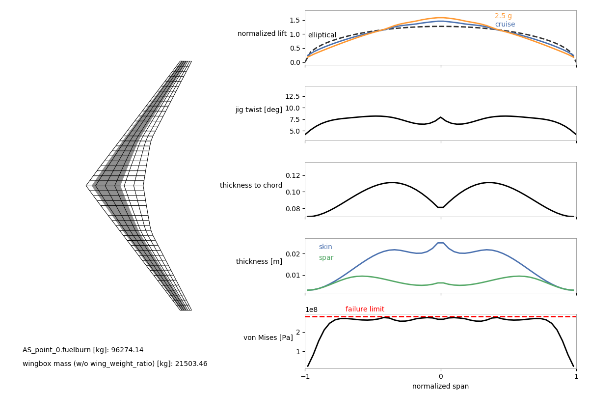
The following are the visualization results (keep in mind that this is with a very large optimization tolerance) for this problem using the plot_wingbox.py visualization script (located in the utils directory). This visualization script requires the .db file as an argument. For example, to use it for this example problem, from the example script’s (wingbox_mpt_opt_example.py) location in the OpenAeroStruct docs directory, we would use:
python ../utils/plot_wingbox.py aerostruct.db
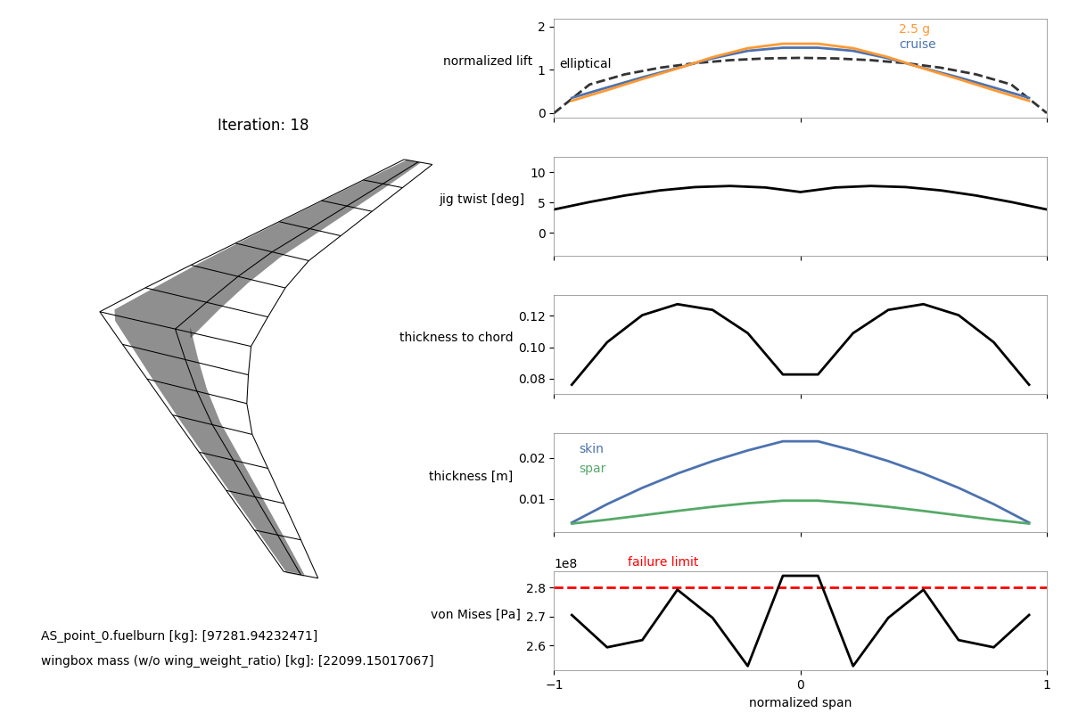
This plotting script currently only works for two-flight-point problems like the one described in this walkthrough.