User-Provided Mesh Example
Here is an example script with a custom mesh provided as an array of coordinates. This should help you understand how meshes are defined in OpenAeroStruct and how to create them for your own custom planform shapes. This is an alternative to the helper-function approach described in Aerodynamic Optimization.
The following shows the portion of the example script in which the user provides the coordinates for the mesh. This example is for a wing with a kink and two distinct trapezoidal segments.
# -----------------------------------------------------------------------------
# CUSTOM MESH: Example mesh for a 2-segment wing with sweep
# -----------------------------------------------------------------------------

# Planform specifications
half_span = 12.0  # wing half-span in m
kink_location = 4.0  # spanwise location of the kink in m

root_chord = 6.0  # root chord in m
kink_chord = 3.0  # kink chord in m
tip_chord = 2.0  # tip chord in m

inboard_LE_sweep = 10.0  # inboard leading-edge sweep angle in deg
outboard_LE_sweep = -10.0  # outboard leading-edge sweep angle in deg

# Mesh specifications
nx = 5  # number of chordwise nodal points (should be odd)
ny_outboard = 9  # number of spanwise nodal points for the outboard segment
ny_inboard = 7  # number of spanwise nodal points for the inboard segment

# Initialize the 3-D mesh object. Indexing: Chordwise, spanwise, then the 3-D coordinates.
# We use ny_inboard+ny_outboard-1 because the 2 segments share the nodes where they connect.
mesh = np.zeros((nx, ny_inboard + ny_outboard - 1, 3))

# The form of this 3-D array can be confusing initially.
# For each node, we are providing the x, y, and z coordinates.
# x is streamwise, y is spanwise, and z is up.
# For example, the node for the leading edge at the tip would be specified as mesh[0, 0, :] = np.array([x, y, z]).
# And the node at the trailing edge at the root would be mesh[nx-1, ny-1, :] = np.array([x, y, z]).
# We only provide the right half of the wing here because we use symmetry.
# Print elements of the mesh to better understand the form.

####### THE Z-COORDINATES ######
# Assume no dihedral, so set the z-coordinate for all the points to 0.
mesh[:, :, 2] = 0.0

####### THE Y-COORDINATES ######
# Using uniform spacing for the spanwise locations of all the nodes within each of the two trapezoidal segments:
# Outboard
mesh[:, :ny_outboard, 1] = np.linspace(half_span, kink_location, ny_outboard)
# Inboard
mesh[:, ny_outboard : ny_outboard + ny_inboard, 1] = np.linspace(kink_location, 0, ny_inboard)[1:]

###### THE X-COORDINATES ######
# Start with the leading edge and create some intermediate arrays that we will use
x_LE = np.zeros(ny_inboard + ny_outboard - 1)

array_for_inboard_leading_edge_x_coord = np.linspace(0, kink_location, ny_inboard) * np.tan(
    inboard_LE_sweep / 180.0 * np.pi
)

array_for_outboard_leading_edge_x_coord = (
    np.linspace(0, half_span - kink_location, ny_outboard) * np.tan(outboard_LE_sweep / 180.0 * np.pi)
    + np.ones(ny_outboard) * array_for_inboard_leading_edge_x_coord[-1]
)

x_LE[:ny_inboard] = array_for_inboard_leading_edge_x_coord
x_LE[ny_inboard : ny_inboard + ny_outboard] = array_for_outboard_leading_edge_x_coord[1:]

# Then the trailing edge
x_TE = np.zeros(ny_inboard + ny_outboard - 1)

array_for_inboard_trailing_edge_x_coord = np.linspace(
    array_for_inboard_leading_edge_x_coord[0] + root_chord,
    array_for_inboard_leading_edge_x_coord[-1] + kink_chord,
    ny_inboard,
)

array_for_outboard_trailing_edge_x_coord = np.linspace(
    array_for_outboard_leading_edge_x_coord[0] + kink_chord,
    array_for_outboard_leading_edge_x_coord[-1] + tip_chord,
    ny_outboard,
)

x_TE[:ny_inboard] = array_for_inboard_trailing_edge_x_coord
x_TE[ny_inboard : ny_inboard + ny_outboard] = array_for_outboard_trailing_edge_x_coord[1:]

# # Quick plot to check leading and trailing edge x-coords
# plt.plot(x_LE, np.arange(0, ny_inboard+ny_outboard-1), marker='*')
# plt.plot(x_TE, np.arange(0, ny_inboard+ny_outboard-1), marker='*')
# plt.show()
# exit()

for i in range(0, ny_inboard + ny_outboard - 1):
    mesh[:, i, 0] = np.linspace(np.flip(x_LE)[i], np.flip(x_TE)[i], nx)

# -----------------------------------------------------------------------------
# END MESH
# -----------------------------------------------------------------------------
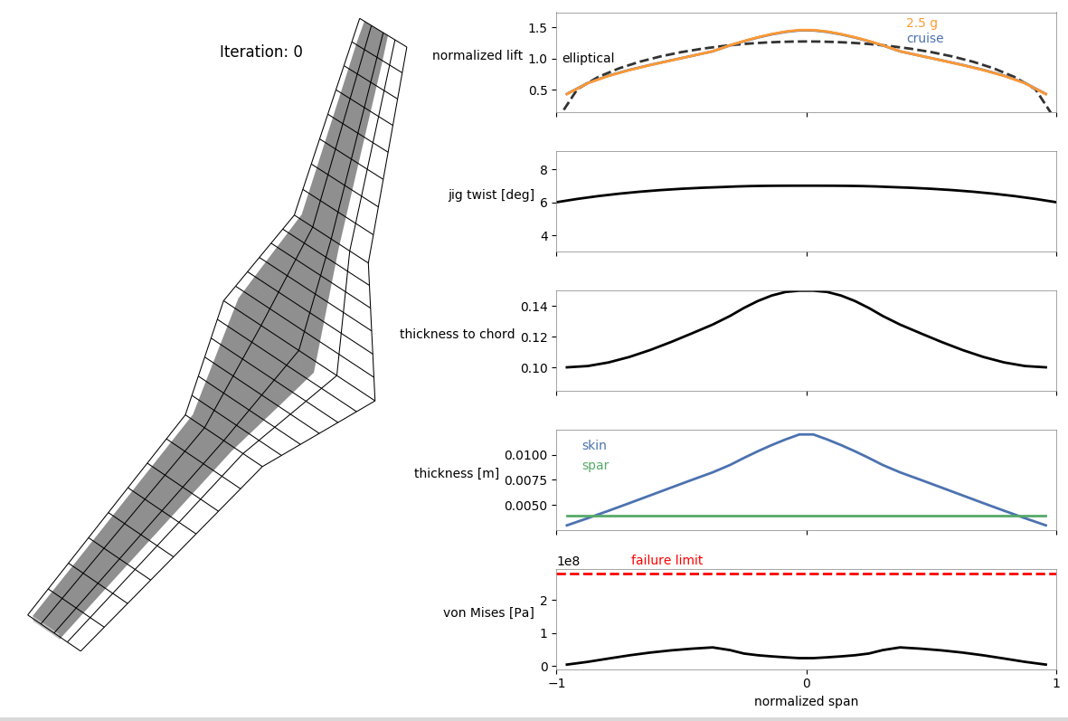
The following shows a visualization of the mesh.
The complete script for the optimization is as follows. Make sure you go through the Aerostructural Optimization with Wingbox before trying to understand this setup.
import warnings
import matplotlib
warnings.filterwarnings('ignore')
matplotlib.use('Agg')
"""
This example script can be used to run a multipoint aerostructural (w/ wingbox) optimization for a custom user-provided mesh.

The fuel burn from the cruise flight-point is the objective function and a 2.5g
maneuver flight-point is used for the structural sizing.
After running the optimization, use the 'plot_wingbox.py' script in the utils/
directory (e.g., as 'python ../utils/plot_wingbox.py aerostruct.db' if running
from this directory) to visualize the results.
'plot_wingbox.py' is still under development and will probably not work as it is for other types of cases for now.
"""

import numpy as np

from openaerostruct.integration.aerostruct_groups import AerostructGeometry, AerostructPoint
from openaerostruct.structures.wingbox_fuel_vol_delta import WingboxFuelVolDelta
import openmdao.api as om


# docs checkpoint 0
# -----------------------------------------------------------------------------
# CUSTOM MESH: Example mesh for a 2-segment wing with sweep
# -----------------------------------------------------------------------------

# Planform specifications
half_span = 12.0  # wing half-span in m
kink_location = 4.0  # spanwise location of the kink in m

root_chord = 6.0  # root chord in m
kink_chord = 3.0  # kink chord in m
tip_chord = 2.0  # tip chord in m

inboard_LE_sweep = 10.0  # inboard leading-edge sweep angle in deg
outboard_LE_sweep = -10.0  # outboard leading-edge sweep angle in deg

# Mesh specifications
nx = 5  # number of chordwise nodal points (should be odd)
ny_outboard = 9  # number of spanwise nodal points for the outboard segment
ny_inboard = 7  # number of spanwise nodal points for the inboard segment

# Initialize the 3-D mesh object. Indexing: Chordwise, spanwise, then the 3-D coordinates.
# We use ny_inboard+ny_outboard-1 because the 2 segments share the nodes where they connect.
mesh = np.zeros((nx, ny_inboard + ny_outboard - 1, 3))

# The form of this 3-D array can be confusing initially.
# For each node, we are providing the x, y, and z coordinates.
# x is streamwise, y is spanwise, and z is up.
# For example, the node for the leading edge at the tip would be specified as mesh[0, 0, :] = np.array([x, y, z]).
# And the node at the trailing edge at the root would be mesh[nx-1, ny-1, :] = np.array([x, y, z]).
# We only provide the right half of the wing here because we use symmetry.
# Print elements of the mesh to better understand the form.

####### THE Z-COORDINATES ######
# Assume no dihedral, so set the z-coordinate for all the points to 0.
mesh[:, :, 2] = 0.0

####### THE Y-COORDINATES ######
# Using uniform spacing for the spanwise locations of all the nodes within each of the two trapezoidal segments:
# Outboard
mesh[:, :ny_outboard, 1] = np.linspace(half_span, kink_location, ny_outboard)
# Inboard
mesh[:, ny_outboard : ny_outboard + ny_inboard, 1] = np.linspace(kink_location, 0, ny_inboard)[1:]

###### THE X-COORDINATES ######
# Start with the leading edge and create some intermediate arrays that we will use
x_LE = np.zeros(ny_inboard + ny_outboard - 1)

array_for_inboard_leading_edge_x_coord = np.linspace(0, kink_location, ny_inboard) * np.tan(
    inboard_LE_sweep / 180.0 * np.pi
)

array_for_outboard_leading_edge_x_coord = (
    np.linspace(0, half_span - kink_location, ny_outboard) * np.tan(outboard_LE_sweep / 180.0 * np.pi)
    + np.ones(ny_outboard) * array_for_inboard_leading_edge_x_coord[-1]
)

x_LE[:ny_inboard] = array_for_inboard_leading_edge_x_coord
x_LE[ny_inboard : ny_inboard + ny_outboard] = array_for_outboard_leading_edge_x_coord[1:]

# Then the trailing edge
x_TE = np.zeros(ny_inboard + ny_outboard - 1)

array_for_inboard_trailing_edge_x_coord = np.linspace(
    array_for_inboard_leading_edge_x_coord[0] + root_chord,
    array_for_inboard_leading_edge_x_coord[-1] + kink_chord,
    ny_inboard,
)

array_for_outboard_trailing_edge_x_coord = np.linspace(
    array_for_outboard_leading_edge_x_coord[0] + kink_chord,
    array_for_outboard_leading_edge_x_coord[-1] + tip_chord,
    ny_outboard,
)

x_TE[:ny_inboard] = array_for_inboard_trailing_edge_x_coord
x_TE[ny_inboard : ny_inboard + ny_outboard] = array_for_outboard_trailing_edge_x_coord[1:]

# # Quick plot to check leading and trailing edge x-coords
# plt.plot(x_LE, np.arange(0, ny_inboard+ny_outboard-1), marker='*')
# plt.plot(x_TE, np.arange(0, ny_inboard+ny_outboard-1), marker='*')
# plt.show()
# exit()

for i in range(0, ny_inboard + ny_outboard - 1):
    mesh[:, i, 0] = np.linspace(np.flip(x_LE)[i], np.flip(x_TE)[i], nx)

# -----------------------------------------------------------------------------
# END MESH
# -----------------------------------------------------------------------------
# docs checkpoint 1


# -----------------------------------------------------------------------------
# On to the problem setup (this is the same setup used for the Q400 example)
# -----------------------------------------------------------------------------

# Provide coordinates for a portion of an airfoil for the wingbox cross-section as an nparray with dtype=complex (to work with the complex-step approximation for derivatives).
# These should be for an airfoil with the chord scaled to 1.
# We use the 10% to 60% portion of the NASA SC2-0612 airfoil for this case
# We use the coordinates available from airfoiltools.com. Using such a large number of coordinates is not necessary.
# The first and last x-coordinates of the upper and lower surfaces must be the same

# fmt: off
upper_x = np.array([0.1, 0.11, 0.12, 0.13, 0.14, 0.15, 0.16, 0.17, 0.18, 0.19, 0.2, 0.21, 0.22, 0.23, 0.24, 0.25, 0.26, 0.27, 0.28, 0.29, 0.3, 0.31, 0.32, 0.33, 0.34, 0.35, 0.36, 0.37, 0.38, 0.39, 0.4, 0.41, 0.42, 0.43, 0.44, 0.45, 0.46, 0.47, 0.48, 0.49, 0.5, 0.51, 0.52, 0.53, 0.54, 0.55, 0.56, 0.57, 0.58, 0.59, 0.6], dtype="complex128")
lower_x = np.array([0.1, 0.11, 0.12, 0.13, 0.14, 0.15, 0.16, 0.17, 0.18, 0.19, 0.2, 0.21, 0.22, 0.23, 0.24, 0.25, 0.26, 0.27, 0.28, 0.29, 0.3, 0.31, 0.32, 0.33, 0.34, 0.35, 0.36, 0.37, 0.38, 0.39, 0.4, 0.41, 0.42, 0.43, 0.44, 0.45, 0.46, 0.47, 0.48, 0.49, 0.5, 0.51, 0.52, 0.53, 0.54, 0.55, 0.56, 0.57, 0.58, 0.59, 0.6], dtype="complex128")
upper_y = np.array([ 0.0447,  0.046,  0.0472,  0.0484,  0.0495,  0.0505,  0.0514,  0.0523,  0.0531,  0.0538, 0.0545,  0.0551,  0.0557, 0.0563,  0.0568, 0.0573,  0.0577,  0.0581,  0.0585,  0.0588,  0.0591,  0.0593,  0.0595,  0.0597,  0.0599,  0.06,    0.0601,  0.0602,  0.0602,  0.0602,  0.0602,  0.0602,  0.0601,  0.06,    0.0599,  0.0598,  0.0596,  0.0594,  0.0592,  0.0589,  0.0586,  0.0583,  0.058,   0.0576,  0.0572,  0.0568,  0.0563,  0.0558,  0.0553,  0.0547,  0.0541], dtype="complex128")  # noqa: E201, E241
lower_y = np.array([-0.0447, -0.046, -0.0473, -0.0485, -0.0496, -0.0506, -0.0515, -0.0524, -0.0532, -0.054, -0.0547, -0.0554, -0.056, -0.0565, -0.057, -0.0575, -0.0579, -0.0583, -0.0586, -0.0589, -0.0592, -0.0594, -0.0595, -0.0596, -0.0597, -0.0598, -0.0598, -0.0598, -0.0598, -0.0597, -0.0596, -0.0594, -0.0592, -0.0589, -0.0586, -0.0582, -0.0578, -0.0573, -0.0567, -0.0561, -0.0554, -0.0546, -0.0538, -0.0529, -0.0519, -0.0509, -0.0497, -0.0485, -0.0472, -0.0458, -0.0444], dtype="complex128")
# fmt: on

surf_dict = {
    # Wing definition
    "name": "wing",  # name of the surface
    "symmetry": True,  # if true, model one half of wing
    "S_ref_type": "wetted",  # how we compute the wing area,
    # can be 'wetted' or 'projected'
    "mesh": mesh,
    "twist_cp": np.array([6.0, 7.0, 7.0, 7.0]),
    "fem_model_type": "wingbox",
    "data_x_upper": upper_x,
    "data_x_lower": lower_x,
    "data_y_upper": upper_y,
    "data_y_lower": lower_y,
    "spar_thickness_cp": np.array([0.004, 0.004, 0.004, 0.004]),  # [m]
    "skin_thickness_cp": np.array([0.003, 0.006, 0.010, 0.012]),  # [m]
    "original_wingbox_airfoil_t_over_c": 0.12,
    # Aerodynamic deltas.
    # These CL0 and CD0 values are added to the CL and CD
    # obtained from aerodynamic analysis of the surface to get
    # the total CL and CD.
    # These CL0 and CD0 values do not vary wrt alpha.
    # They can be used to account for things that are not included, such as contributions from the fuselage, nacelles, tail surfaces, etc.
    "CL0": 0.0,
    "CD0": 0.0142,
    "with_viscous": True,  # if true, compute viscous drag
    "with_wave": True,  # if true, compute wave drag
    # Airfoil properties for viscous drag calculation
    "k_lam": 0.05,  # percentage of chord with laminar
    # flow, used for viscous drag
    "c_max_t": 0.38,  # chordwise location of maximum thickness
    "t_over_c_cp": np.array([0.1, 0.1, 0.15, 0.15]),
    # Structural values are based on aluminum 7075
    "E": 73.1e9,  # [Pa] Young's modulus
    "G": (73.1e9 / 2 / 1.33),  # [Pa] shear modulus (calculated using E and the Poisson's ratio here)
    "yield": 420.0e6,  # [Pa] yield stress
    "safety_factor": 1.5,  # safety factor
    "mrho": 2.78e3,  # [kg/m^3] material density
    "strength_factor_for_upper_skin": 1.0,  # the yield stress is multiplied by this factor for the upper skin
    "wing_weight_ratio": 1.25,
    "exact_failure_constraint": False,  # if false, use KS function
    "struct_weight_relief": True,
    "distributed_fuel_weight": True,
    "fuel_density": 803.0,  # [kg/m^3] fuel density (only needed if the fuel-in-wing volume constraint is used)
    "Wf_reserve": 500.0,  # [kg] reserve fuel mass
}

surfaces = [surf_dict]

# Create the problem and assign the model group
prob = om.Problem()

# Add problem information as an independent variables component
indep_var_comp = om.IndepVarComp()
indep_var_comp.add_output("v", val=np.array([0.5 * 310.95, 0.3 * 340.294]), units="m/s")
indep_var_comp.add_output("alpha", val=0.0, units="deg")
indep_var_comp.add_output("alpha_maneuver", val=0.0, units="deg")
indep_var_comp.add_output("Mach_number", val=np.array([0.5, 0.3]))
indep_var_comp.add_output(
    "re",
    val=np.array([0.569 * 310.95 * 0.5 * 1.0 / (1.56 * 1e-5), 1.225 * 340.294 * 0.3 * 1.0 / (1.81206 * 1e-5)]),
    units="1/m",
)
indep_var_comp.add_output("rho", val=np.array([0.569, 1.225]), units="kg/m**3")
indep_var_comp.add_output("CT", val=0.43 / 3600, units="1/s")
indep_var_comp.add_output("R", val=2e6, units="m")
indep_var_comp.add_output("W0", val=25400 + surf_dict["Wf_reserve"], units="kg")
indep_var_comp.add_output("speed_of_sound", val=np.array([310.95, 340.294]), units="m/s")
indep_var_comp.add_output("load_factor", val=np.array([1.0, 2.5]))
indep_var_comp.add_output("empty_cg", val=np.zeros((3)), units="m")
indep_var_comp.add_output("fuel_mass", val=3000.0, units="kg")

prob.model.add_subsystem("prob_vars", indep_var_comp, promotes=["*"])

# Loop over each surface in the surfaces list
for surface in surfaces:
    # Get the surface name and create a group to contain components
    # only for this surface
    name = surface["name"]

    aerostruct_group = AerostructGeometry(surface=surface)

    # Add group to the problem with the name of the surface.
    prob.model.add_subsystem(name, aerostruct_group)

# Loop through and add a certain number of aerostruct points
for i in range(2):
    point_name = "AS_point_{}".format(i)
    # Connect the parameters within the model for each aerostruct point

    # Create the aero point group and add it to the model
    AS_point = AerostructPoint(surfaces=surfaces, internally_connect_fuelburn=False)

    prob.model.add_subsystem(point_name, AS_point)

    # Connect flow properties to the analysis point
    prob.model.connect("v", point_name + ".v", src_indices=[i])
    prob.model.connect("Mach_number", point_name + ".Mach_number", src_indices=[i])
    prob.model.connect("re", point_name + ".re", src_indices=[i])
    prob.model.connect("rho", point_name + ".rho", src_indices=[i])
    prob.model.connect("CT", point_name + ".CT")
    prob.model.connect("R", point_name + ".R")
    prob.model.connect("W0", point_name + ".W0")
    prob.model.connect("speed_of_sound", point_name + ".speed_of_sound", src_indices=[i])
    prob.model.connect("empty_cg", point_name + ".empty_cg")
    prob.model.connect("load_factor", point_name + ".load_factor", src_indices=[i])
    prob.model.connect("fuel_mass", point_name + ".total_perf.L_equals_W.fuelburn")
    prob.model.connect("fuel_mass", point_name + ".total_perf.CG.fuelburn")

    for surface in surfaces:
        name = surface["name"]

        if surf_dict["distributed_fuel_weight"]:
            prob.model.connect("load_factor", point_name + ".coupled.load_factor", src_indices=[i])

        com_name = point_name + "." + name + "_perf."
        prob.model.connect(
            name + ".local_stiff_transformed", point_name + ".coupled." + name + ".local_stiff_transformed"
        )
        prob.model.connect(name + ".nodes", point_name + ".coupled." + name + ".nodes")

        # Connect aerodynamic mesh to coupled group mesh
        prob.model.connect(name + ".mesh", point_name + ".coupled." + name + ".mesh")
        if surf_dict["struct_weight_relief"]:
            prob.model.connect(name + ".element_mass", point_name + ".coupled." + name + ".element_mass")

        # Connect performance calculation variables
        prob.model.connect(name + ".nodes", com_name + "nodes")
        prob.model.connect(name + ".cg_location", point_name + "." + "total_perf." + name + "_cg_location")
        prob.model.connect(name + ".structural_mass", point_name + "." + "total_perf." + name + "_structural_mass")

        # Connect wingbox properties to von Mises stress calcs
        prob.model.connect(name + ".Qz", com_name + "Qz")
        prob.model.connect(name + ".J", com_name + "J")
        prob.model.connect(name + ".A_enc", com_name + "A_enc")
        prob.model.connect(name + ".htop", com_name + "htop")
        prob.model.connect(name + ".hbottom", com_name + "hbottom")
        prob.model.connect(name + ".hfront", com_name + "hfront")
        prob.model.connect(name + ".hrear", com_name + "hrear")

        prob.model.connect(name + ".spar_thickness", com_name + "spar_thickness")
        prob.model.connect(name + ".t_over_c", com_name + "t_over_c")

prob.model.connect("alpha", "AS_point_0" + ".alpha")
prob.model.connect("alpha_maneuver", "AS_point_1" + ".alpha")

# Here we add the fuel volume constraint componenet to the model
prob.model.add_subsystem("fuel_vol_delta", WingboxFuelVolDelta(surface=surface))
prob.model.connect("wing.struct_setup.fuel_vols", "fuel_vol_delta.fuel_vols")
prob.model.connect("AS_point_0.fuelburn", "fuel_vol_delta.fuelburn")

if surf_dict["distributed_fuel_weight"]:
    prob.model.connect("wing.struct_setup.fuel_vols", "AS_point_0.coupled.wing.struct_states.fuel_vols")
    prob.model.connect("fuel_mass", "AS_point_0.coupled.wing.struct_states.fuel_mass")

    prob.model.connect("wing.struct_setup.fuel_vols", "AS_point_1.coupled.wing.struct_states.fuel_vols")
    prob.model.connect("fuel_mass", "AS_point_1.coupled.wing.struct_states.fuel_mass")

comp = om.ExecComp("fuel_diff = (fuel_mass - fuelburn) / fuelburn", units="kg")
prob.model.add_subsystem("fuel_diff", comp, promotes_inputs=["fuel_mass"], promotes_outputs=["fuel_diff"])
prob.model.connect("AS_point_0.fuelburn", "fuel_diff.fuelburn")


## Use these settings if you do not have pyOptSparse or SNOPT
prob.driver = om.ScipyOptimizeDriver()
prob.driver.options["optimizer"] = "SLSQP"
prob.driver.options["tol"] = 1e-4

recorder = om.SqliteRecorder("aerostruct.db")
prob.driver.add_recorder(recorder)

# We could also just use prob.driver.recording_options['includes']=['*'] here, but for large meshes the database file becomes extremely large. So we just select the variables we need.
prob.driver.recording_options["includes"] = [
    "alpha",
    "rho",
    "v",
    "cg",
    "AS_point_1.cg",
    "AS_point_0.cg",
    "AS_point_0.coupled.wing_loads.loads",
    "AS_point_1.coupled.wing_loads.loads",
    "AS_point_0.coupled.wing.normals",
    "AS_point_1.coupled.wing.normals",
    "AS_point_0.coupled.wing.widths",
    "AS_point_1.coupled.wing.widths",
    "AS_point_0.coupled.aero_states.wing_sec_forces",
    "AS_point_1.coupled.aero_states.wing_sec_forces",
    "AS_point_0.wing_perf.CL1",
    "AS_point_1.wing_perf.CL1",
    "AS_point_0.coupled.wing.S_ref",
    "AS_point_1.coupled.wing.S_ref",
    "wing.geometry.twist",
    "wing.mesh",
    "wing.skin_thickness",
    "wing.spar_thickness",
    "wing.t_over_c",
    "wing.structural_mass",
    "AS_point_0.wing_perf.vonmises",
    "AS_point_1.wing_perf.vonmises",
    "AS_point_0.coupled.wing.def_mesh",
    "AS_point_1.coupled.wing.def_mesh",
]

prob.driver.recording_options["record_objectives"] = True
prob.driver.recording_options["record_constraints"] = True
prob.driver.recording_options["record_desvars"] = True
prob.driver.recording_options["record_inputs"] = True

prob.model.add_objective("AS_point_0.fuelburn", scaler=1e-5)

prob.model.add_design_var("wing.twist_cp", lower=-15.0, upper=15.0, scaler=0.1)
prob.model.add_design_var("wing.spar_thickness_cp", lower=0.003, upper=0.1, scaler=1e2)
prob.model.add_design_var("wing.skin_thickness_cp", lower=0.003, upper=0.1, scaler=1e2)
prob.model.add_design_var("wing.geometry.t_over_c_cp", lower=0.07, upper=0.2, scaler=10.0)
prob.model.add_design_var("fuel_mass", lower=0.0, upper=2e5, scaler=1e-5)
prob.model.add_design_var("alpha_maneuver", lower=-15.0, upper=15)

prob.model.add_constraint("AS_point_0.CL", equals=0.6)
prob.model.add_constraint("AS_point_1.L_equals_W", equals=0.0)
prob.model.add_constraint("AS_point_1.wing_perf.failure", upper=0.0)

prob.model.add_constraint("fuel_vol_delta.fuel_vol_delta", lower=0.0)
prob.model.add_constraint("fuel_diff", equals=0.0)

# Set up the problem
prob.setup()
/home/docs/checkouts/readthedocs.org/user_builds/mdolab-openaerostruct/envs/latest/lib/python3.11/site-packages/openmdao/core/system.py:2769: PromotionWarning:'AS_point_0.coupled.wing.struct_states' <class SpatialBeamStates>: input variable 'load_factor', promoted using 'load_factor', was already promoted using 'load_factor'.
/home/docs/checkouts/readthedocs.org/user_builds/mdolab-openaerostruct/envs/latest/lib/python3.11/site-packages/openmdao/core/system.py:2769: PromotionWarning:'AS_point_0.coupled.wing.struct_states' <class SpatialBeamStates>: input variable 'nodes', promoted using 'nodes', was already promoted using 'nodes'.
/home/docs/checkouts/readthedocs.org/user_builds/mdolab-openaerostruct/envs/latest/lib/python3.11/site-packages/openmdao/core/system.py:2769: PromotionWarning:'AS_point_1.coupled.wing.struct_states' <class SpatialBeamStates>: input variable 'load_factor', promoted using 'load_factor', was already promoted using 'load_factor'.
/home/docs/checkouts/readthedocs.org/user_builds/mdolab-openaerostruct/envs/latest/lib/python3.11/site-packages/openmdao/core/system.py:2769: PromotionWarning:'AS_point_1.coupled.wing.struct_states' <class SpatialBeamStates>: input variable 'nodes', promoted using 'nodes', was already promoted using 'nodes'.
/home/docs/checkouts/readthedocs.org/user_builds/mdolab-openaerostruct/envs/latest/lib/python3.11/site-packages/openmdao/core/driver.py:780: OpenMDAOWarning:ScipyOptimizeDriver: No matches for pattern 'cg' in recording_options['includes'].
# change linear solver for aerostructural coupled adjoint
prob.model.AS_point_0.coupled.linear_solver = om.LinearBlockGS(iprint=0, maxiter=30, use_aitken=True)
prob.model.AS_point_1.coupled.linear_solver = om.LinearBlockGS(iprint=0, maxiter=30, use_aitken=True)

# om.view_model(prob)

# prob.check_partials(form='central', compact_print=True)

prob.run_driver()
==================
AS_point_0.coupled
==================
NL: NLBGS 1 ; 55907.3939 1
NL: NLBGS 2 ; 59181.5774 1.05856441
NL: NLBGS 3 ; 1932.61109 0.0345680769
NL: NLBGS 4 ; 49.803332 0.000890818343
NL: NLBGS 5 ; 0.126112452 2.25573835e-06
NL: NLBGS 6 ; 0.00519590448 9.29376978e-08
NL: NLBGS 7 ; 4.25351023e-05 7.6081354e-10
NL: NLBGS 8 ; 5.51007761e-08 9.85572251e-13
NL: NLBGS Converged

==================
AS_point_1.coupled
==================
NL: NLBGS 1 ; 60763.1469 1
NL: NLBGS 2 ; 54750.9315 0.901054904
NL: NLBGS 3 ; 1645.63616 0.0270828
NL: NLBGS 4 ; 39.2586228 0.000646092653
NL: NLBGS 5 ; 0.0926805548 1.52527576e-06
NL: NLBGS 6 ; 0.00346780579 5.70708722e-08
NL: NLBGS 7 ; 2.9946882e-05 4.92846134e-10
NL: NLBGS 8 ; 3.11009028e-08 5.1183825e-13
NL: NLBGS Converged

==================
AS_point_0.coupled
==================
NL: NLBGS 1 ; 1.45169908e-09 1
NL: NLBGS Converged

==================
AS_point_1.coupled
==================
NL: NLBGS 1 ; 8.75825779e-10 1
NL: NLBGS Converged

==================
AS_point_0.coupled
==================
NL: NLBGS 1 ; 12273.9529 1
NL: NLBGS 2 ; 12097.8639 0.985653438
NL: NLBGS 3 ; 1919.773 0.156410328
NL: NLBGS 4 ; 83.0974049 0.00677022355
NL: NLBGS 5 ; 0.936851159 7.63283978e-05
NL: NLBGS 6 ; 0.0805543593 6.56303312e-06
NL: NLBGS 7 ; 0.0020818039 1.69611527e-07
NL: NLBGS 8 ; 2.43472839e-05 1.98365467e-09
NL: NLBGS 9 ; 1.55064412e-06 1.26336164e-10
NL: NLBGS 10 ; 1.25990898e-07 1.02648999e-11
NL: NLBGS 11 ; 4.58788263e-09 3.73790145e-13
NL: NLBGS Converged

==================
AS_point_1.coupled
==================
NL: NLBGS 1 ; 93132.2815 1
NL: NLBGS 2 ; 98281.9356 1.05529398
NL: NLBGS 3 ; 16302.9416 0.175051457
NL: NLBGS 4 ; 888.340076 0.00953847648
NL: NLBGS 5 ; 33.0462271 0.00035483107
NL: NLBGS 6 ; 1.61200642 1.73087827e-05
NL: NLBGS 7 ; 0.0550717032 5.91327758e-07
NL: NLBGS 8 ; 0.00296757518 3.18640877e-08
NL: NLBGS 9 ; 4.66060264e-05 5.00428269e-10
NL: NLBGS 10 ; 9.7335059e-06 1.04512697e-10
NL: NLBGS 11 ; 1.71551054e-06 1.84201495e-11
NL: NLBGS 12 ; 4.07775355e-08 4.37845341e-13
NL: NLBGS Converged

==================
AS_point_0.coupled
==================
NL: NLBGS 1 ; 4705.65519 1
NL: NLBGS 2 ; 4949.89921 1.05190436
NL: NLBGS 3 ; 547.001821 0.116243498
NL: NLBGS 4 ; 23.3512345 0.00496237688
NL: NLBGS 5 ; 0.142469491 3.02762283e-05
NL: NLBGS 6 ; 0.0102175417 2.17133242e-06
NL: NLBGS 7 ; 0.000177344301 3.76874833e-08
NL: NLBGS 8 ; 9.47682054e-07 2.01392158e-10
NL: NLBGS 9 ; 6.00837891e-08 1.27684215e-11
NL: NLBGS Converged

==================
AS_point_1.coupled
==================
NL: NLBGS 1 ; 11390.5012 1
NL: NLBGS 2 ; 11452.4394 1.0054377
NL: NLBGS 3 ; 1727.30403 0.151644251
NL: NLBGS 4 ; 53.4080096 0.00468881998
NL: NLBGS 5 ; 0.324755012 2.85110379e-05
NL: NLBGS 6 ; 0.0365863558 3.21200579e-06
NL: NLBGS 7 ; 0.00061574305 5.40575905e-08
NL: NLBGS 8 ; 1.04694363e-05 9.19137454e-10
NL: NLBGS 9 ; 5.23673401e-07 4.59745705e-11
NL: NLBGS 10 ; 1.92269845e-08 1.68798406e-12
NL: NLBGS Converged

==================
AS_point_0.coupled
==================
NL: NLBGS 1 ; 7777.64092 1
NL: NLBGS 2 ; 8362.13151 1.07515011
NL: NLBGS 3 ; 623.169995 0.0801232664
NL: NLBGS 4 ; 46.5318118 0.00598276679
NL: NLBGS 5 ; 0.163401121 2.10090852e-05
NL: NLBGS 6 ; 0.00405005347 5.20730323e-07
NL: NLBGS 7 ; 0.00024761016 3.18361523e-08
NL: NLBGS 8 ; 6.97350254e-07 8.9660896e-11
NL: NLBGS 9 ; 1.25040409e-08 1.60769069e-12
NL: NLBGS Converged

==================
AS_point_1.coupled
==================
NL: NLBGS 1 ; 7686.14124 1
NL: NLBGS 2 ; 7765.71393 1.01035275
NL: NLBGS 3 ; 865.120344 0.112555874
NL: NLBGS 4 ; 51.3449622 0.00668020019
NL: NLBGS 5 ; 0.377906663 4.91672806e-05
NL: NLBGS 6 ; 0.0135986828 1.76924706e-06
NL: NLBGS 7 ; 0.000607549273 7.90447709e-08
NL: NLBGS 8 ; 3.2212246e-06 4.1909516e-10
NL: NLBGS 9 ; 1.11429524e-07 1.44974598e-11
NL: NLBGS 10 ; 7.3397502e-09 9.54933037e-13
NL: NLBGS Converged

==================
AS_point_0.coupled
==================
NL: NLBGS 1 ; 3019.68828 1
NL: NLBGS 2 ; 3220.68238 1.06656121
NL: NLBGS 3 ; 234.874306 0.0777809777
NL: NLBGS 4 ; 18.2114791 0.00603091359
NL: NLBGS 5 ; 0.0699118987 2.31520251e-05
NL: NLBGS 6 ; 0.00136219987 4.51106123e-07
NL: NLBGS 7 ; 9.00156391e-05 2.98095799e-08
NL: NLBGS 8 ; 2.11253242e-07 6.99586258e-11
NL: NLBGS 9 ; 3.70728511e-09 1.22770457e-12
NL: NLBGS Converged

==================
AS_point_1.coupled
==================
NL: NLBGS 1 ; 3093.11331 1
NL: NLBGS 2 ; 2991.68285 0.967207649
NL: NLBGS 3 ; 242.455288 0.0783855177
NL: NLBGS 4 ; 22.1582824 0.00716374741
NL: NLBGS 5 ; 0.143769535 4.64805266e-05
NL: NLBGS 6 ; 0.000948574828 3.06673159e-07
NL: NLBGS 7 ; 7.11334207e-05 2.29973537e-08
NL: NLBGS 8 ; 1.04428276e-07 3.37615424e-11
NL: NLBGS 9 ; 1.25607401e-09 4.06087294e-13
NL: NLBGS Converged

==================
AS_point_0.coupled
==================
NL: NLBGS 1 ; 1935.91934 1
NL: NLBGS 2 ; 2074.60153 1.07163635
NL: NLBGS 3 ; 141.918131 0.0733078739
NL: NLBGS 4 ; 11.4592359 0.0059192734
NL: NLBGS 5 ; 0.0448884783 2.31871635e-05
NL: NLBGS 6 ; 0.000604191002 3.12095132e-07
NL: NLBGS 7 ; 4.29281313e-05 2.21745454e-08
NL: NLBGS 8 ; 9.75535785e-08 5.03913445e-11
NL: NLBGS Converged

==================
AS_point_1.coupled
==================
NL: NLBGS 1 ; 1980.78384 1
NL: NLBGS 2 ; 1963.30586 0.991176232
NL: NLBGS 3 ; 147.798753 0.074616296
NL: NLBGS 4 ; 13.6653491 0.00689896034
NL: NLBGS 5 ; 0.0885546602 4.47068774e-05
NL: NLBGS 6 ; 0.00068974086 3.48216118e-07
NL: NLBGS 7 ; 5.19301916e-05 2.62169908e-08
NL: NLBGS 8 ; 6.10830766e-08 3.08378307e-11
NL: NLBGS Converged

==================
AS_point_0.coupled
==================
NL: NLBGS 1 ; 27.2948914 1
NL: NLBGS 2 ; 23.7012013 0.868338363
NL: NLBGS 3 ; 2.07444231 0.0760011197
NL: NLBGS 4 ; 0.139894625 0.00512530431
NL: NLBGS 5 ; 0.000867912938 3.17976329e-05
NL: NLBGS 6 ; 2.80928377e-05 1.02923427e-06
NL: NLBGS 7 ; 1.43366698e-06 5.25251028e-08
NL: NLBGS 8 ; 3.68307107e-09 1.34936278e-10
NL: NLBGS Converged

==================
AS_point_1.coupled
==================
NL: NLBGS 1 ; 51.4407961 1
NL: NLBGS 2 ; 33.8909559 0.658834204
NL: NLBGS 3 ; 0.879992133 0.0171068918
NL: NLBGS 4 ; 0.0907107688 0.00176340134
NL: NLBGS 5 ; 0.000893143456 1.73625512e-05
NL: NLBGS 6 ; 1.73192755e-05 3.36683661e-07
NL: NLBGS 7 ; 1.34623045e-06 2.61704824e-08
NL: NLBGS 8 ; 1.52783582e-09 2.97008587e-11
NL: NLBGS Converged
Optimization terminated successfully    (Exit mode 0)
            Current function value: 0.027924147979429468
            Iterations: 6
            Function evaluations: 7
            Gradient evaluations: 6
Optimization Complete
-----------------------------------

==================
AS_point_0.coupled
==================
NL: NLBGS 1 ; 24029.0727 1
NL: NLBGS 2 ; 0 0
NL: NLBGS Converged

==================
AS_point_1.coupled
==================
NL: NLBGS 1 ; 57060.1783 1
NL: NLBGS 2 ; 0 0
NL: NLBGS Converged
# prob.run_model()
print("The fuel burn value is", prob["AS_point_0.fuelburn"][0], "[kg]")
The fuel burn value is 2792.4147979429467 [kg]
print(
    "The wingbox mass (excluding the wing_weight_ratio) is",
    prob["wing.structural_mass"][0] / surf_dict["wing_weight_ratio"],
    "[kg]",
)
The wingbox mass (excluding the wing_weight_ratio) is 1158.9598707326968 [kg]
There is plenty of room for improvement. A finer mesh and a tighter optimization tolerance should be used.